Category Archives: Risk

Chart of the distributions of Portfolio’s nominal returns and residual returns used to detect evidence of investment skill as well as the test statistics

How Much Time is Needed to Detect Evidence of Investment Skill?

A recent MarketWatch piece cited a talk in Hong Kong by Economics Nobel Prize winner Professor Robert Merton wherein he discussed the challenges of evaluating investment managers. The following article assumes that the above summary of Professor Merton’s talk is accurate. The piece, and assumedly the talk, argued that, given typical nominal portfolio returns and volatilities, it takes impractically long to detect evidence of investment skill. The argument claimed to prove that all manager selection is futile. Instead, it proved that naïve nominal performance metrics are of little use.

Any test of the effectiveness of manager selection is also a test of the analytical process that distills skill. That nominal investment performance is primarily due to factor (systematic, market) noise and thus reverts is well-known. It is thus unsurprising to find flaws in an approach to manager selection that is as antiquated as Ptolemaic Astronomy.

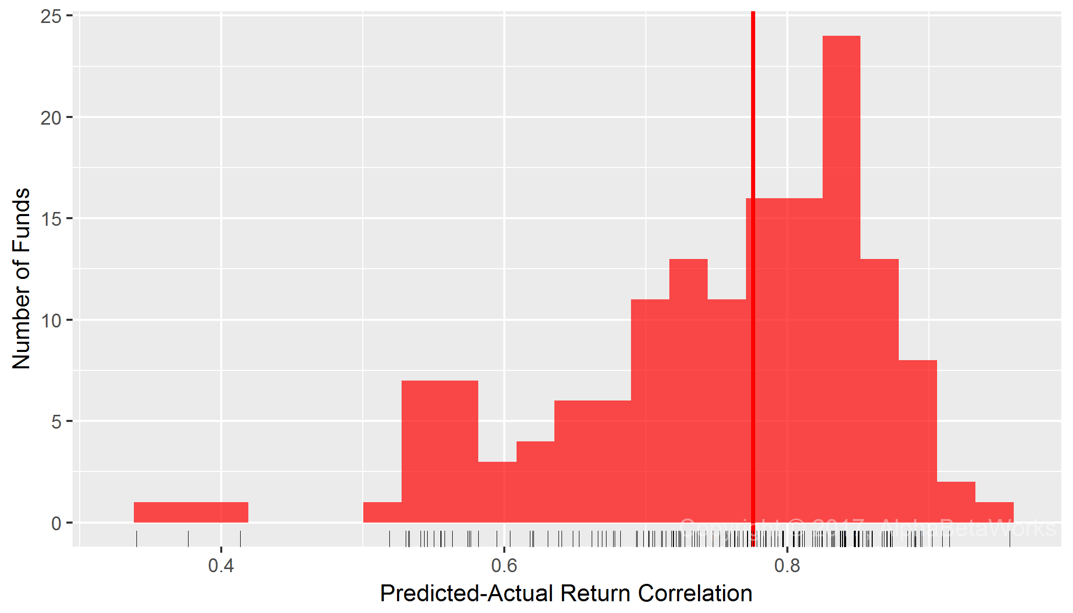
In this article, we will illustrate the difference between a naïve attempt to detect evidence of investment skill using nominal returns and a more productive effort relying on alphas (residual, security selection, stock picking returns) isolated using a capable modern multi-factor equity risk model. Whereas the former approach is futile at best, the latter approach is successful. In fact, rather than taking decades, a capable modern system can identify skill with high confidence in months.

Detecting Evidence of Investment Skill Using Nominal Returns

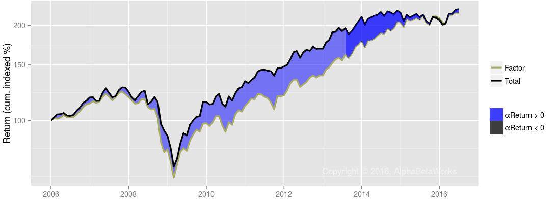
Consider nominal returns of a Portfolio and a Benchmark. The Portfolio is a live long-only fund implementing a Smart Beta active investment strategy:

Chart of the absolute cumulative returns for the Portfolio and the Benchmark as well as Portfolio’s cumulative return relative to the Benchmark

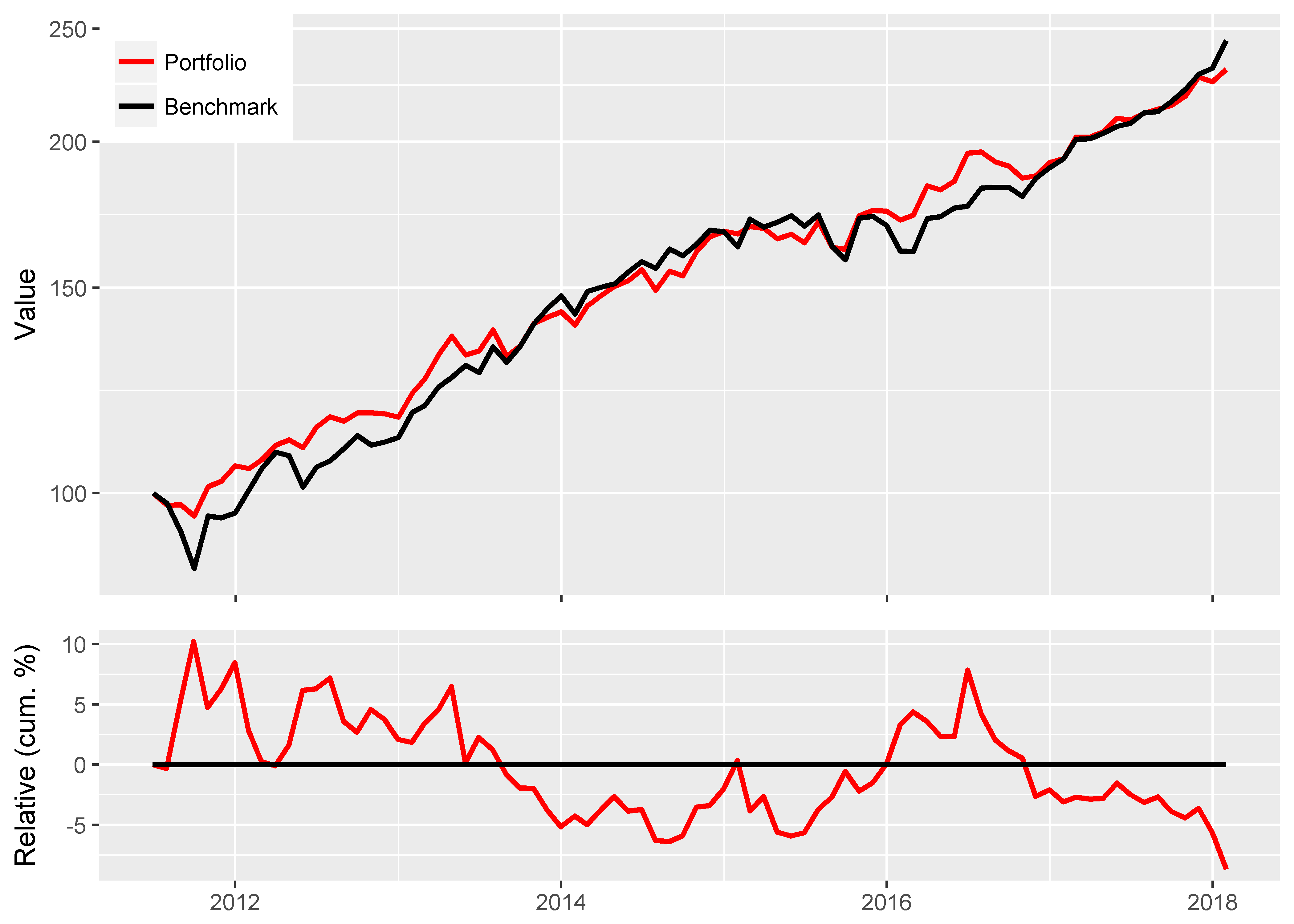
Portfolio’s and Benchmark’s Cumulative Returns

                           Portfolio Benchmark
 Annualized Return            0.1336    0.1433
 Annualized Std Dev           0.0879    0.1093
 Annualized Sharpe (Rf=0%)    1.5194    1.3115

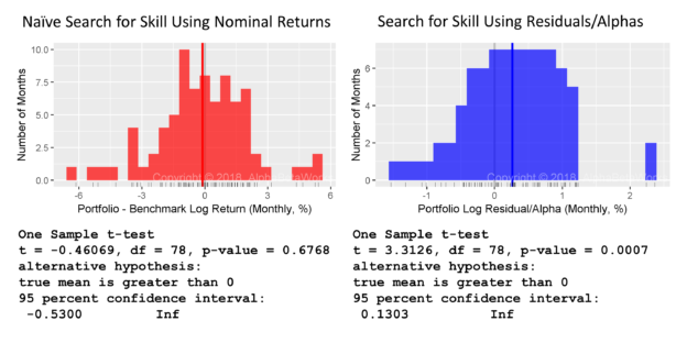
With a heroic assumption that log returns follow a normal distribution, a t-test appears to confirm Professor Merton’s argument. Even with over six years of data, the returns are too noisy for a statistical inference:

Chart of the distribution of Portfolio’s returns relative to the Benchmark used to detect evidence of investment skill

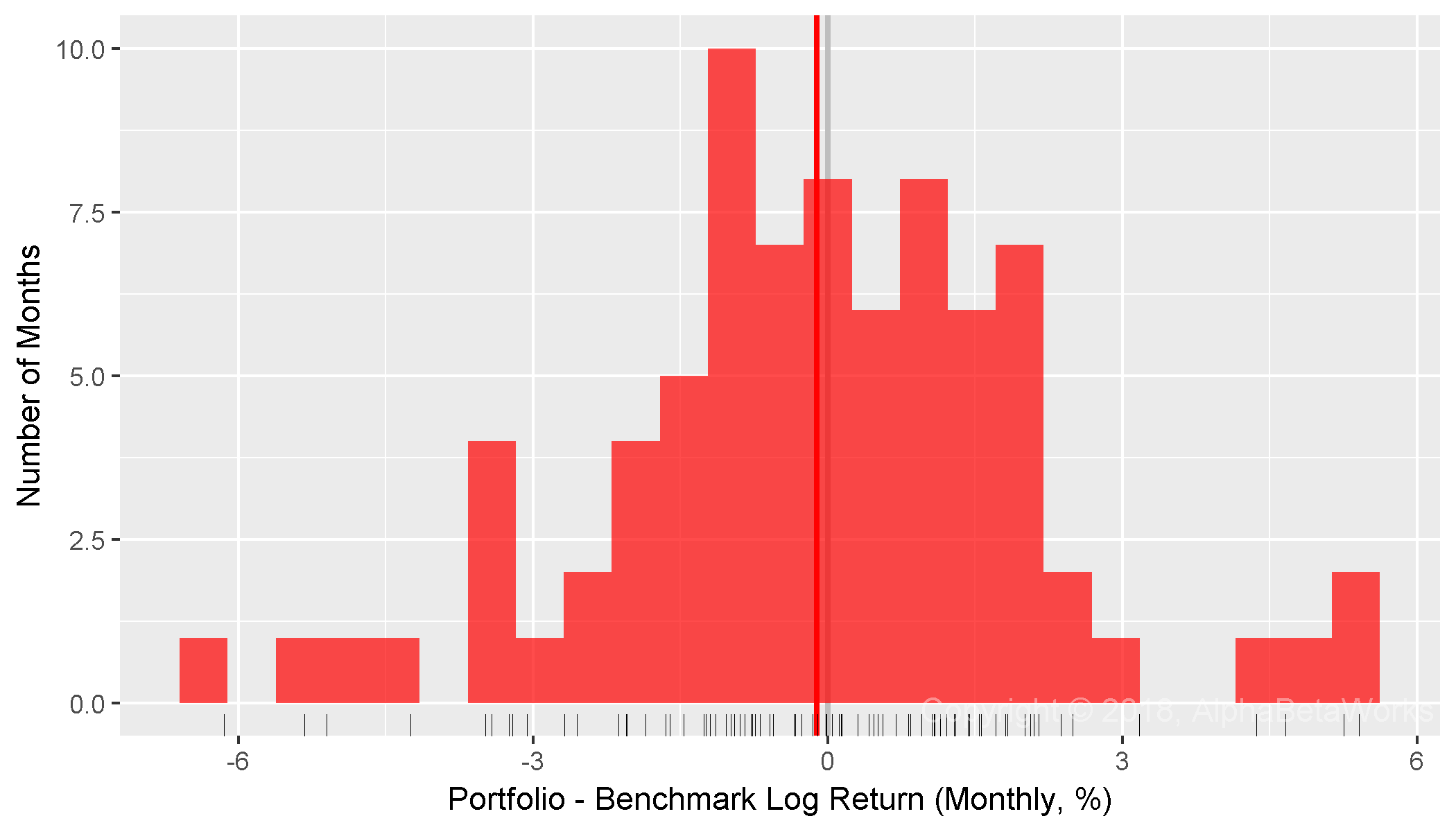
Distribution of Portfolio’s Returns Relative to the Benchmark

    Min. 1st Qu.  Median    Mean 3rd Qu.    Max. 
 -6.1441 -1.2186 -0.0201 -0.1149  1.2481  5.4068 
 
      One Sample t-test
 t = -0.4607, df = 78, p-value = 0.6768
 alternative hypothesis: true mean is greater than 0
 95 percent confidence interval:
  -0.5300        Inf

Detecting Evidence of Investment Skill Using Alphas/Residuals

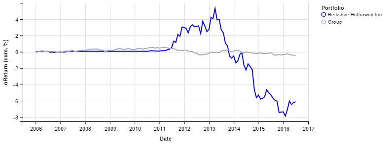
By comparison, consider the same Portfolio’s residual returns, or alphas, for the same period, isolated with the AlphaBetaWorks’ standard Long-Horizon Statistical U.S. Equity Risk Model. These are also the returns Portfolio would have generated if its factor exposures had been fully hedged (its returns factor-neutralized, or residualized) using the Model:

Chart of the absolute cumulative residual (alpha, security selection, stock picking returns) for the Portfolio

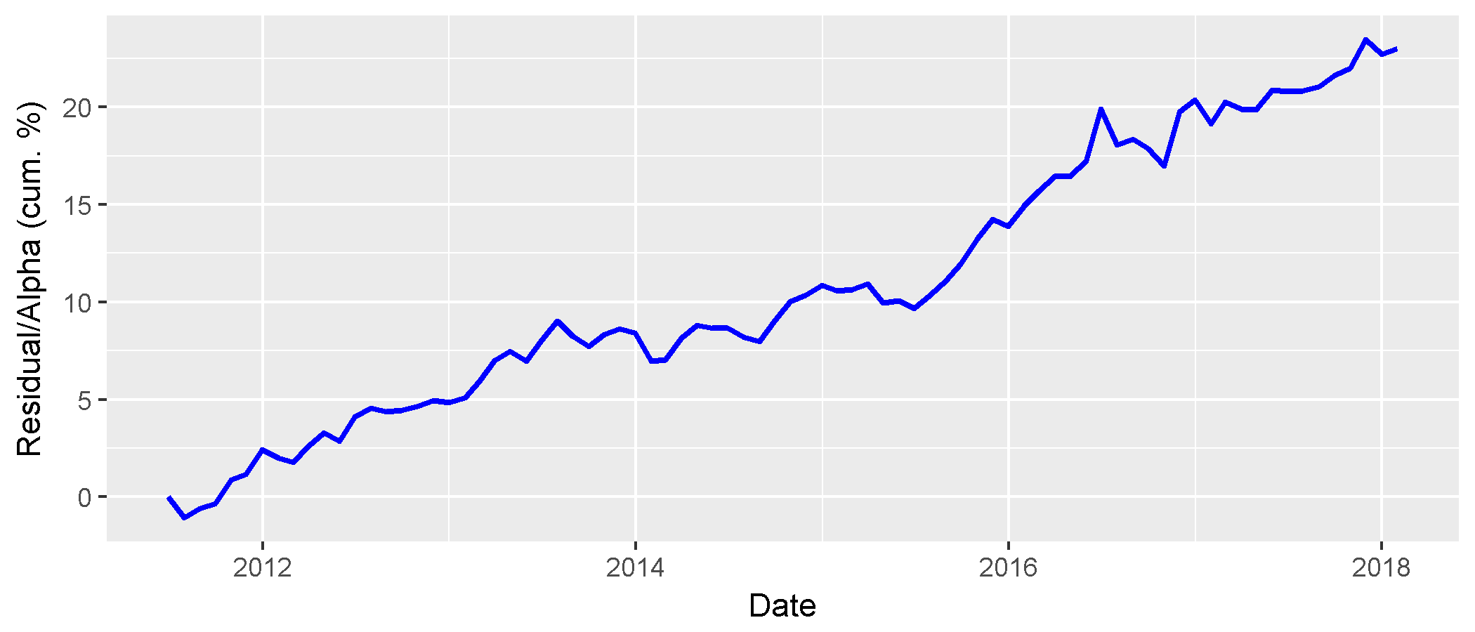
Portfolio’s Cumulative Residual/Alpha

With an equally questionable assumption that log residuals follow a normal distribution, a t-test is now highly statistically significant:

Chart of the distribution of Portfolio’s residual returns used to detect evidence of investment skill

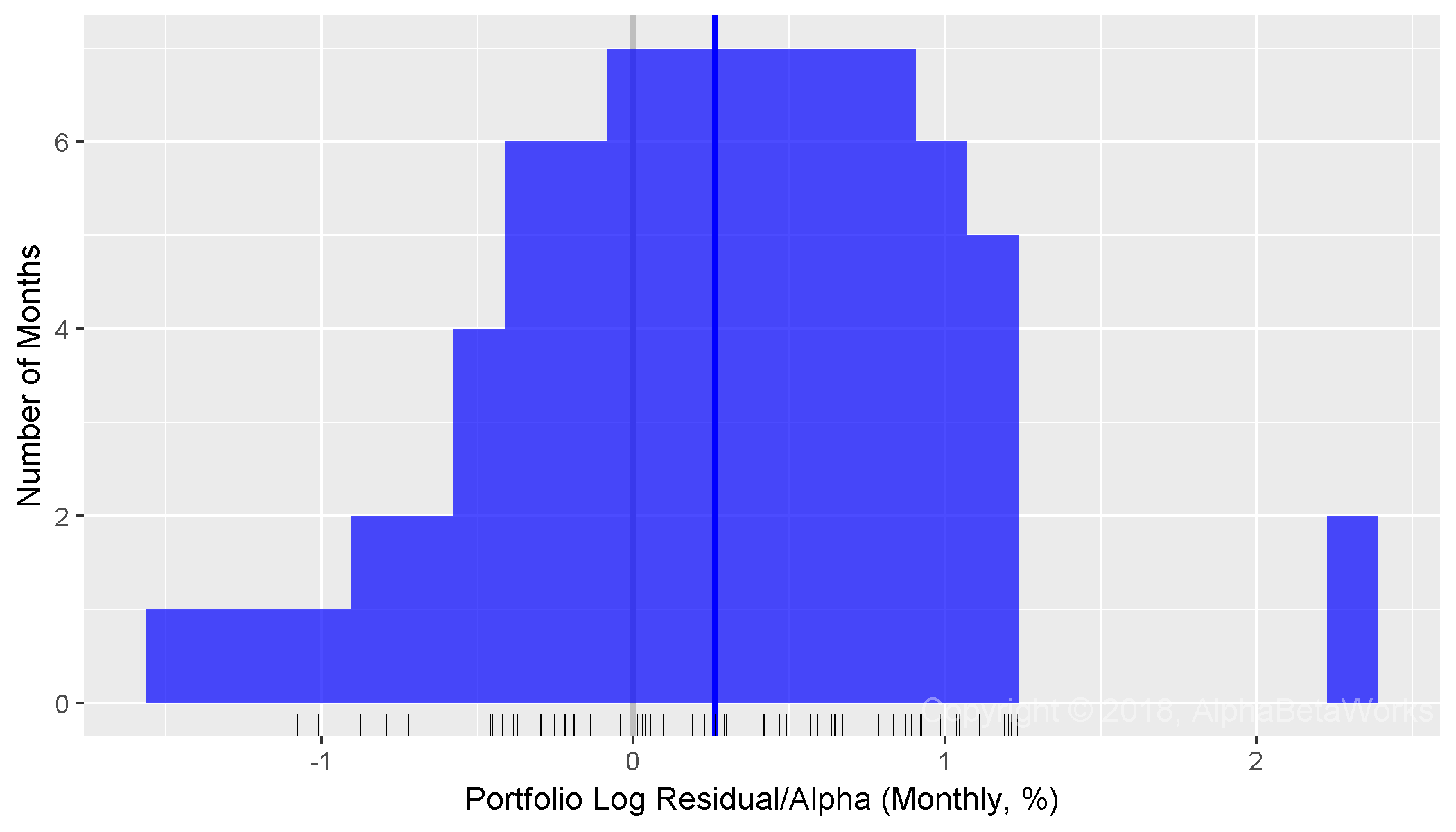
Distribution of the Portfolio’s Residuals/Alphas 

    Min. 1st Qu.  Median    Mean 3rd Qu.    Max. 
 -1.5300 -0.2064  0.2643  0.2620  0.7289  2.3663 
 
      One Sample t-test
 t = 3.3126, df = 78, p-value = 0.0007
 alternative hypothesis: true mean is greater than 0
 95 percent confidence interval:
  0.1303         Inf

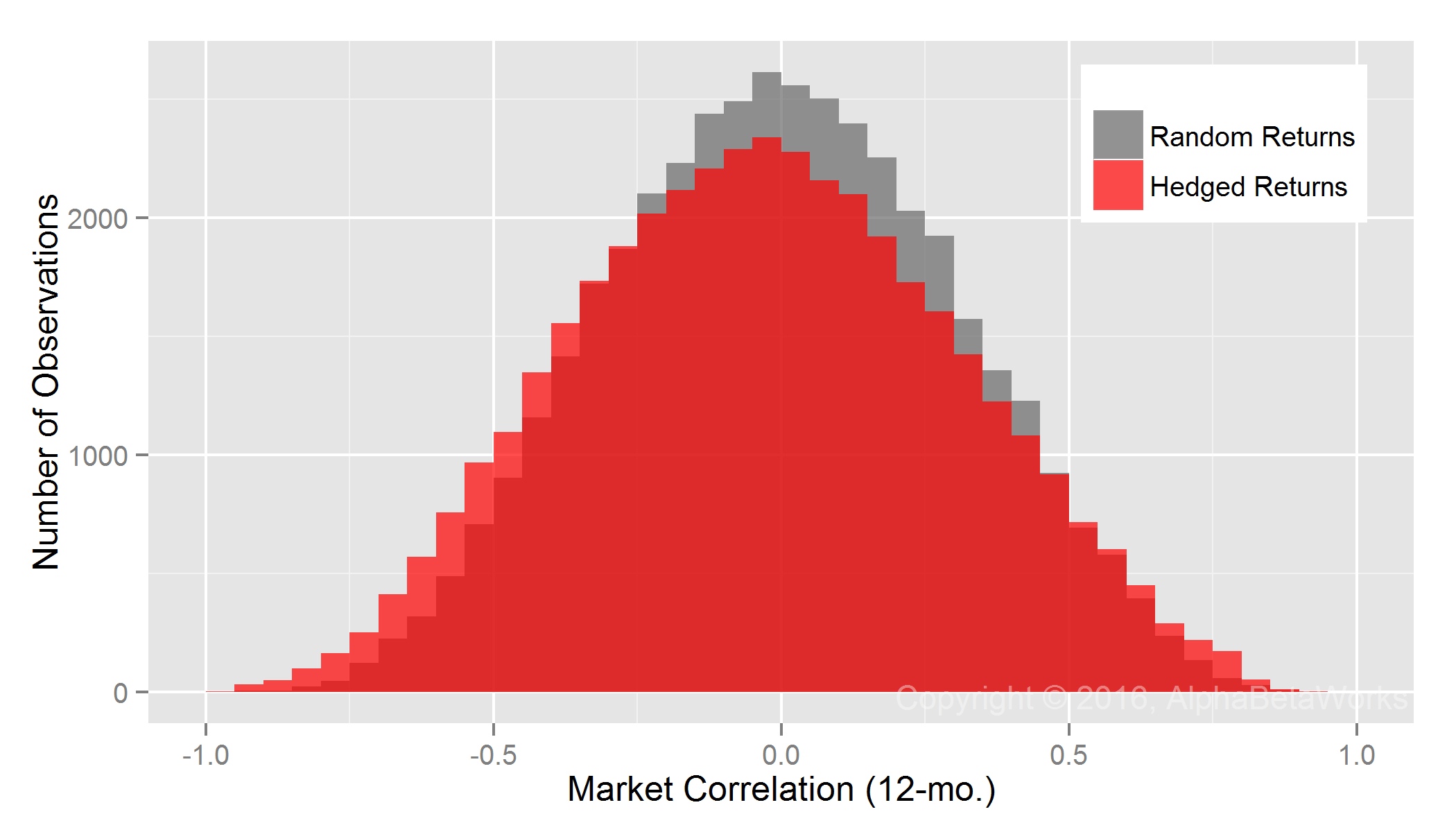
Whereas Professor Merton’s argument does indeed apply to nominal returns, it does not apply to their residuals. A critical difference is the lower dispersion of residual returns. Over 90% of the variance of a typical active equity portfolio is due to factor exposures rather than to stock picking. Therefore, using nominal returns to measure skill is like trying to take a baby’s temperature by examining her bath water, rather than the baby herself.

Whereas at least 67 out of 100 monkeys picking stocks at random are expected to outperform the Portfolio, less than 1 out of 1,000 is expected to generate higher residuals – a highly statistically significant result. Thus, with the help of a capable equity risk model, strong evidence of skill can be identified in months rather than in decades.

Converting Residuals into Nominal Outperformance

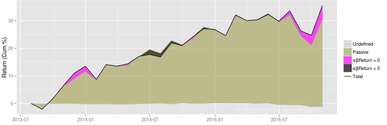
Assuming the equity risk model uses investable factors, as AlphaBetaWorks’s models do, the residual return stream above is investable. In fact, in the idealized case of costless leverage, positive residual returns can be turned into outperformance relative to any benchmark. Below is the performance of Portfolio after it is hedged to match the factor exposures of the Benchmark. The evidence of skill is now plainly visible in the naïve absolute and relative nominal return metrics:

Chart of the absolute cumulative returns for the Portfolio hedged to match the factor exposures of the Benchmark, the Benchmark, as well as Portfolio’s cumulative return relative to the Benchmark

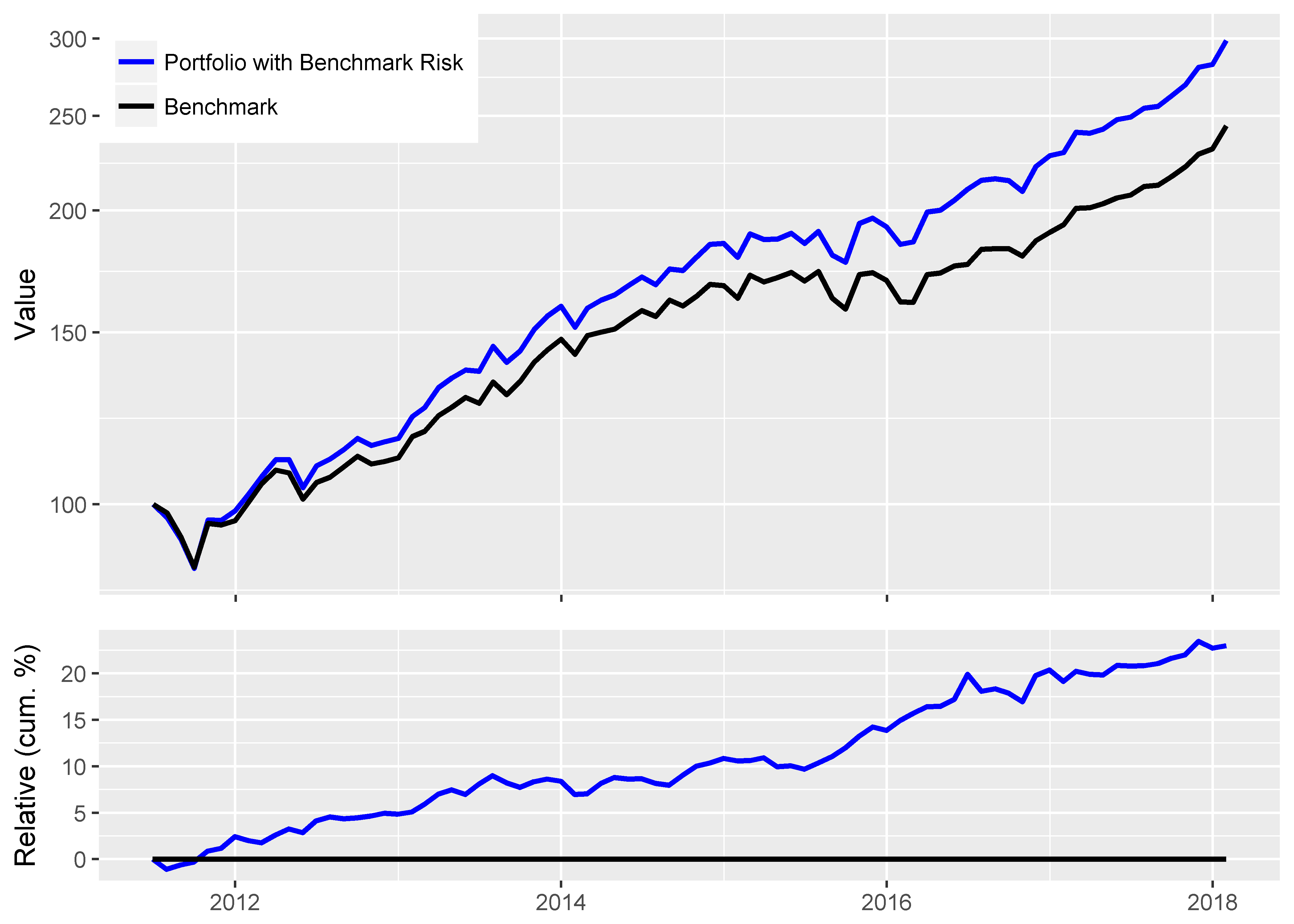
Cumulative Returns for the Portfolio Hedged to Match the Benchmark and the Benchmark

                          Portfolio with Benchmark Risk  Benchmark
 Annualized Return                                0.1784    0.1433
 Annualized Std Dev                               0.1168    0.1093
 Annualized Sharpe (Rf=0%)                        1.5276    1.3115

Conclusions

  • Since factor noise dominates nominal returns, the use of nominal returns to detect evidence of investment skill takes far too long to be practical.
  • After distilling stock picking performance (alphas, residual returns) from factor noise, statistically significant evidence of investment skill can become evident in months, rather than in decades.
  • Hedging makes it possible to turn positive stock picking returns into nominal outperformance with respect to any benchmark.
The information herein is not represented or warranted to be accurate, correct, complete or timely.
Past performance is no guarantee of future results.
Copyright © 2012-2018, AlphaBetaWorks, a division of Alpha Beta Analytics, LLC. All rights reserved.
Content may not be republished without express written consent.

What Fraction of International Smart Beta Tracking Error is Dumb Beta?

In earlier articles, we showed that the returns of most U.S. and international smart beta ETFs are primarily due to their dumb beta (dumb factor) exposures. Thus, smart beta ETFs turn out to actively time dumb beta factors. In fact, most smart beta strategies are primarily different approaches to sector rotation. After readers’ requests to extend the above analysis to relative returns and tracking error, we showed that the findings hold for U.S. smart beta tracking error. This article extends the analysis to international smart beta tracking error.

The results hold for international smart beta tracking error: Though some international smart beta ETFs do provide valuable exposures to idiosyncratic factors, most primarily re-shuffle basic dumb Region and Sector Factors.  In fact, dumb beta exposures are even more influential for international smart beta equity ETFs than for their U.S. peers. Most international smart beta equity ETFs are mainly region and sector rotation strategies in disguise. Consequently, investors and allocators must guard against fancy re-packaging of dumb international risk factors as smart beta and should perform rigorous region and sector factor analysis of their smart beta allocations. Further, many international smart beta strategies can be substantially replicated and blended using simple passive Region and Sector Factors.

Measuring the Influence of Dumb Beta Factors on International Smart Beta ETFs

We used the same dataset of International Smart Beta Equity ETFs as our earlier article on international smart beta ETFs’ dumb factor exposures. We estimated monthly positions of each ETF and then used these positions to calculate portfolio factor exposures to traditional factors such as Regions and Sectors.  These ex-ante factor exposures at the end of month m1 were used to predict returns during the subsequent month m2. We then calculated predicted and actual returns relative to the Global Equity Market (defined as the iShares MSCI ACWI Index Fund – ACWI). The correlation between actual and predicted relative returns quantified the influence of dumb beta factors on smart beta tracking error. The higher the correlation, the more similar a smart beta ETF is to a portfolio of traditional, simple, and dumb systematic risk factors.

The Influence of Region Beta on International Smart Beta ETFs

The simplest systematic risk factor to describe each security is its Region (Region Market Beta). Region Beta measures exposure to one of 10 broad regional equity markets (e.g., North America, Developing Asia). These are the most basic and cheap passive international factors. Even this single-factor model estimated with robust statistical techniques delivered 0.67 mean and 0.68 median correlations between predicted and actual relative returns:

Chart of the correlations between relative returns of replicating portfolios constructed using Region Factors and actual relative returns for international smart beta equity ETFs

International Smart Beta Equity ETFs: Correlation between relative returns predicted using Region Factors and actual relative returns

  Min. 1st Qu.  Median    Mean 3rd Qu.    Max. 
0.2490  0.5662  0.6791  0.6655  0.7805  0.9185

For a quarter of smart beta ETFs, Region Factor alone replicates 61% (0.7805²) of tracking error. For this group of strategies, international smart beta tracking error is largely due to region rotation.

The Influence of Region and Sector Betas on International Smart Beta ETFs

We next extended the model with Sector Factors. Sector Beta measures exposure to one of 10 broad sectors (e.g., Energy, Technology). Region and Sector Betas, estimated with robust methods, delivered 0.75 mean and 0.77 median correlations between predicted and actual relative returns:

Chart of the correlations between relative returns of replicating portfolios constructed using Region and Sector Factors and actual relative returns for international smart beta equity ETFs

International Smart Beta Equity ETFs: Correlation between relative returns predicted using Region and Sector Factors and actual relative returns

  Min. 1st Qu.  Median    Mean 3rd Qu.    Max. 
0.2604  0.6807  0.7673  0.7461  0.8523  0.9494

For most international smart beta ETFs, Region and Sector Factors replicate 59% (0.7673²) of tracking error. Thus, for most international smart beta equity ETFs, over half of tracking error is due to region and sector rotation.

International Smart Beta Variance and International Dumb Beta Variance

Rather than measure correlations between relative returns of replicating dumb beta portfolios and ETFs, we can instead measure the fractions of their (relative) variances unexplained by dumb beta exposures. The Dumb Beta Variance (in red below) is the distribution of ETFs’ relative variances due to their dumb Region and Sector Factor exposures. The Smart Beta Variance (in blue below) is the distribution of ETFs’ relative variances unrelated to their dumb beta exposures:

Chart of the percentage of international smart beta tracking error explained by traditional, non-smart, or dumb beta Region and Sector Factors and the percentage of tracking error unexplained by these factors for international smart beta equity ETFs

International Equity Smart Beta ETFs: Percentage of tracking error explained and unexplained by the Region and Sector dumb beta exposures

Percentage of international equity smart beta ETFs’ relative variances due to dumb beta exposures:

Min. 1st Qu.  Median    Mean 3rd Qu.    Max. 
6.78   46.34   58.88   57.70   72.65   90.13

Percentage of international equity smart beta ETFs’ relative variances unrelated to dumb beta exposures:

Min. 1st Qu.  Median    Mean 3rd Qu.    Max. 
9.87   27.35   41.12   42.30   53.66   93.22

For a quarter of strategies, over 2/3 of international smart beta tracking error is due to region and sector rotation, and for some, it reaches 90%.

Our analysis focused on the most basic Region and Sector Factors and excluded Value/Growth and Size Factors, which are decades old and also considered dumb beta by some. If one expands the list of dumb beta factors, smart beta variance shrinks further.

Conclusions

  • Traditional, or dumb, Region and Sector Betas account for the majority of international smart beta tracking error.
  • Smart beta effects, unexplained by the traditional Region and Sector Betas, account for 41% of variance or less for most international smart beta ETFs.
  • With proper analytics, investors and allocators can identify products that do provide unique international smart beta exposures and can guard against fancy re-packaging of dumb international beta.
  • Investors and allocators can monitor the majority of international smart beta ETF relative risk by focusing on their Region and Sector Factor exposures.
  • Most international smart beta strategies can be combined using Region and Sector Factor portfolios.
The information herein is not represented or warranted to be accurate, correct, complete or timely.
Past performance is no guarantee of future results.
Copyright © 2012-2017, AlphaBetaWorks, a division of Alpha Beta Analytics, LLC. All rights reserved.
Content may not be republished without express written consent.

What Fraction of Smart Beta Tracking Error is Dumb Beta?

Our earlier articles discussed how some smart beta strategies turn out to be merely high beta strategies and how others actively time the market. We also showed that, for the majority of smart beta ETFs, returns are mostly attributable to the traditional dumb Market and Sector Factors. Consequently, the absolute performance of most smart beta strategies can be substantially captured by sector rotation. We received questions about these studies’ focus on absolute performance: The attribution of absolute performance to the Market and Sector factors tells little about tracking error and relative variance. Perhaps smart beta volatility is attributable to dumb factors, but smart beta tracking error is not?

This article addresses the above criticism and analyzes smart beta tracking error rather than (absolute) volatility. The results hold: Though some smart beta ETFs do provide valuable exposures to idiosyncratic factors, most primarily re-shuffle basic dumb factors. Whether one considers their absolute or relative performance, most smart beta equity ETFs are largely sector rotation strategies in disguise. Consequently, investors and allocators must guard against elaborate re-packaging of dumb factors as smart beta and perform rigorous sector and industry analysis of their smart beta allocations. Further, dozens of smart beta strategies can be substantially replicated and blended using simple sector factor portfolios.

Measuring the Influence of Dumb Beta Factors on Smart Beta ETFs

We used the same U.S. Smart Beta ETF dataset as our earlier study of smart beta ETFs’ dumb factor exposures. For each ETF, we estimated monthly positions and then used these positions to calculate portfolio factor exposures for traditional (dumb beta) factors such as Market and Sectors.  The ex-ante factor exposures at the end of each month were used to predict the following month’s returns. The correlation between actual and predicted returns relative to the U.S. Equity Market (defined as the iShares Russell 3000 ETF – IWV) quantified the influence of dumb beta factors on smart beta tracking error. The higher the correlation, the more similar a smart beta ETF is to a portfolio of traditional, simple, and dumb systematic risk factors.

The Influence of Market Beta on Smart Beta ETFs

Our simplest test used a single systematic risk factor – Market Beta. Median correlation between predicted and actual relative returns of smart beta ETFs was 0.31:

Chart of the correlations between predicted relative returns constructed using a single Market factor and actual relative historical returns for over 200 U.S. smart beta equity ETFs

U.S. Smart Beta Equity ETFs: Correlation between predicted relative returns and actual relative returns using a single Market factor

   Min. 1st Qu.  Median    Mean 3rd Qu.    Max. 
-0.1089  0.2129  0.3050  0.3096  0.4053  0.8899

The influence of Market Beta on tracking error is much lower than its influence on absolute variance since it only measures relative performance due to deviations from Market’s risk.

The Influence of Market and Sector Betas on Smart Beta ETFs

We next tested a two-factor model that added a Sector Factor. Each security belonged to one of 10 broad sectors (e.g., Energy, Technology). Market and Sector Betas, estimated with robust methods, delivered 0.68 mean and median correlations between predicted and actual relative returns of smart beta ETFs:

Chart of the correlations between predicted relative returns constructed using Market and Sector factors and actual historical returns for over 200 U.S. smart beta equity ETFs

U.S. Smart Beta Equity ETFs: Correlation between predicted relative returns and actual relative returns using Market and Sector factors

  Min. 1st Qu.  Median    Mean 3rd Qu.    Max. 
0.0355  0.5983  0.6821  0.6801  0.7981  0.9630

Put differently: For most broad U.S. equity smart beta ETFs, U.S. Market and Sector Betas alone account for approximately half of tracking error and relative variance.

The Influence of all Dumb Factor Betas on Smart Beta ETFs

For the final tests, we added additional dumb factors such as Bonds, Value, and Size. All dumb factor betas delivered 0.74 mean and 0.78 median correlations between predicted and actual relative returns of smart beta ETFs:

Chart of the correlations between predicted relative returns constructed using dumb risk factors and actual historical returns for over 200 U.S. smart beta equity ETFs

U.S. Smart Beta Equity ETFs: Correlation between predicted relative returns and actual relative returns using dumb beta factors

  Min. 1st Qu.  Median    Mean 3rd Qu.    Max. 
0.2094  0.6875  0.7759  0.7447  0.8387  0.9715

Thus, for most broad U.S. equity smart beta ETFs, dumb beta factors account for the majority of tracking error.

Smart Beta Tracking Error and Dumb Beta Tracking Error

Rather than measure correlations between relative returns predicted by dumb beta exposures and actual relative returns, we can instead measure the fraction of relative variance unexplained by dumb beta exposures. This value (in blue below) is the fraction of smart beta tracking error that is unrelated to dumb beta factors:

Chart of the percentage of tracking error or variance explained by traditional, non-smart, or dumb beta factors and the percentage of tracking error unexplained by these factors for over 200 U.S. smart beta equity ETFs

Percentage of Smart Beta Tracking Error Explained and Unexplained by Dumb Beta Factors

Percentage of Tracking Error Explained by Dumb Beta Factors

 Min. 1st Qu.  Median    Mean 3rd Qu.    Max. 
4.384  47.268  60.197  57.141  70.346  94.381

Percentage of Tracking Error Unexplained by Dumb Beta Factors

 Min. 1st Qu.  Median    Mean 3rd Qu.    Max. 
5.619  29.654  39.803  42.859  52.732  95.616

Conclusions

  • Dumb factor exposures are responsible for over 60% of the smart beta tracking error for most strategies.
  • Market and Sector Factors alone account for half of the tracking error for most U.S. equity smart beta ETFs.
  • Most smart beta strategies can be viewed as (largely) various approaches to sector rotation. They can also be substantially replicated and blended using sector rotation.
The information herein is not represented or warranted to be accurate, correct, complete or timely.
Past performance is no guarantee of future results.
Copyright © 2012-2017, AlphaBetaWorks, a division of Alpha Beta Analytics, LLC. All rights reserved.
Content may not be republished without express written consent.
 

Berkshire Hathaway’s Alpha Decay

Berkshire’s Recent Exposure and Performance Raise Questions

There is a good reason many investors consider Berkshire Hathaway the paragon of investment success. For over 20 years, Berkshire’s equity portfolio has outperformed the general market on a risk-adjusted basis. But, in the past two years Berkshire’s alpha has turned negative. We identify the principal culprit and provide evidence of style drift at Berkshire – either by Warren Buffett or one of his possible successors.

Berkshire Hathaway Security Selection Return

Below is a chart showing Berkshire’s long equity portfolio performance since 2006, during which time it gained 108%. Many investors and guru-followers will dig no further. But simplistic analysis produces dangerous conclusions. Much of Berkshire’s performance—and that of most stocks—can be attributed to systematic sources, or factors. Berkshire’s nominal performance is influenced by the Market, bond rates, and FX rates. Since factor returns revert, and nominal returns are a contrarian indicator of future performance, it is important to separate Berkshire’s factor performance from its stock-picking skill.

We use the AlphaBetaWorks Statistical Equity Risk Model to analyze Berkshire’s equity portfolio since 2006. The chart below shows Berkshire returns due to systematic (factor) and idiosyncratic (stock selection, alpha) components.

Chart of the Factor and Stock Selection Components of Berkshire Hathaway's Long Equity Portfolio Returns

Berkshire Hathaway Long Equity Portfolio Performance – Factor and Stock Selection Components

In the chart above, the black line represents Berkshire’s long equity portfolio total return. Within this, the gray line is performance due to factors, and the blue area reflects Berkshire’s positive returns from stock selection, or αReturn. Since “alpha” and security selection performance are widely and often inconsistently used, AlphaBetaWorks defines a rigorous metric of security selection performance as αReturn, which is performance net of all factor effects, or the return a portfolio would have generated if markets were flat.

From 2006 to 2013 Berkshire’s return from stock selection alone was +29.9%. But in 2014 Berkshire’s αReturn started to decline (thinning blue area). Between 2014 and 2015, Berkshire’s return from stock selection was -16.3%.

Whereas the chart above depicts Berkshire αReturn including factor returns, the chart below depicts Berkshire’s ten-year αReturn in isolation.

Chart of the cumulative Return from Stock Selection (αReturn) of Berkshire Hathaway

Berkshire Hathaway Return from Stock Selection (αReturn)

Berkshire’s αReturn began to decay in 2014. There is one principal sector responsible for this: Technology.

Berkshire Hathaway Technology Exposure

Berkshire made a significant bet in the technology sector in mid-2011 after having avoided it for a very long time:

Chart of the historical technology factor exposure of Berkshire Hathaway Long Equity portfolio

Berkshire Hathaway Long Equity Factor Exposure – Technology

From 2006 to 2011, Berkshire’s technology exposure was effectively zero. But starting in 2011 it went up dramatically.

Berkshire Hathaway Technology Security Selection

This bet has gone poorly. In fact, this sector is the principal contributor to Berkshire’s recent αReturn decay:

Chart of the cumulative Return from Stock Selection (αReturn) of Berkshire Hathaway technology portfolio

Berkshire Hathaway Return from Stock Selection (αReturn) – Technology Sector

Berkshire’s long equity portfolio suffered over a 12% loss from technology stock selection, peak-to-trough.

Style Drift, Succession Issues?

Warren Buffett has long been very public about his avoidance of technology investments, citing reluctance to allocate capital to a business he cannot understand. So why was a manager with no record in, and known skepticism towards, the technology industry making large bets in it? In this light, the above data indicates worrying style drift. Perhaps this large technology sector bet was made by one of his likely successors, which raises an equally important question about manager succession and the style drift risk therein: does a new portfolio manager demonstrate security selection skill (positive αReturn) in general, and in the areas of growing allocation like technology? And what other changes should investors expect of new leadership?

Whether Berkshire’s recent negative αReturn is Buffett’s own error or commission or a byproduct of portfolio manager transition is beyond the scope of this piece. Our focus is identifying active return, its sources (factor timing, stock selection), and their predictive value. All of the above lead to improved performance. In Berkshire’s case, our approach has identified that an established star manager shifted focus to an area previously avoided (technology), and that this shift reduced stock selection performance. Whatever the reason, the results are troublesome. Their early warnings are critical to investors’ and managers’ performance.

Such analysis of risk and performance using holdings data and a predictive equity risk model provides indicators that enhance manager/fund selection and future performance. It can also highlight emerging issues, such as style drift.

Summary

  • After a long, positive run, Berkshire Hathaway’s stock selection returns (alpha) turned negative in 2014.
  • Berkshire’s allocation to the technology sector was the principal driver behind its recent negative alpha.
  • Whether by Buffett or someone new, style drift is a cause of Berkshire’s increased allocation to technology and the resulting negative alpha.
  • Even when investing in or alongside star managers, it is critical that investors and allocators rely on robust and predictive tools to detect early signs of style drift and stock selection decay.
The information herein is not represented or warranted to be accurate, correct, complete or timely.
Past performance is no guarantee of future results.
Copyright © 2012-2016, AlphaBetaWorks, a division of Alpha Beta Analytics, LLC. All rights reserved.
Content may not be republished without express written consent.

Tests of Equity Market Hedging: U.S. Hedge Funds

Our earlier piece tested several equity market hedging techniques on U.S. equity mutual fund portfolios. We now extend the tests to U.S. hedge fund long equity portfolios. Since these are generally less diversified and more active than mutual funds, simplistic approaches that use a fixed 100% short (1 beta) or rely on returns-based style analysis (RBSA) fail even more dramatically for hedge funds. Yet, a robust statistical equity risk model applied to portfolio holdings remains close to the ideal of perfect hedging. A robust and well-tested technique is thus even more vital for managing hedge fund exposures.

Equity Market Hedging Techniques

We analyze approximately 600 hedge fund long U.S. equity portfolios that are tractable from regulatory filings. Note that roughly half of U.S. hedge fund portfolios are impossible to analyze accurately due to the quarterly data frequency and high turnover. Similarly to our earlier analysis of mutual fund portfolio hedging, we evaluate three approaches to calculating market hedge ratios:

  • Constant 100% market exposure (1 beta): This common ad-hoc approach used by portfolio managers and analytics vendors supposes that all portfolios have the same risk as a benchmark or a hedge.
  • Returns-based style analysis (RBSA): This statistical approach estimates portfolio factor exposures by regressing portfolio returns against factor returns.
  • Statistical equity risk model applied to portfolio holdings: A more statistically and algorithmically intensive technique estimates factor exposures of positions, essentially performing RBSA on individual stocks, and aggregates these to calculate portfolio factor exposures.

Our study spans 10 years. We calculate hedge ratios at the end of each month and use these to hedge portfolios during the following month. This produces a series of 10-year realized (ex-post) hedged portfolio returns. We further break these series into 12-month intervals and calculate their correlations to the Market. Low average market correlation and low dispersion of correlations indicates that a hedging technique effectively eliminates systematic market exposure of a typical portfolio.

Realized Market Correlations of Hedged Hedge Fund Portfolios

Realized Market Correlations of Random Return Series

A large return dataset, even when perfectly random, will contain some subsets with high market correlations. To control for this, we generate random return samples (observations) and calculate their market correlations. These results, attainable only with a perfect hedge, are the standard against which we evaluate equity market hedging techniques:

Chart of the correlations between 12-month random return series and 12-month returns of U.S. Equity Market, with sample size chosen to match the hedge fund dataset, used as a baseline for equity market hedging effectiveness.

Realized 12-month market correlations of random return series

   Min. 1st Qu.  Median    Mean 3rd Qu.    Max.
-0.9374 -0.2157 -0.0001  0.0022  0.2173  0.9190

Realized Market Correlations of Portfolios Hedged using a 100% Market Short

As with mutual funds, the assumption that all hedge fund long equity portfolios’ market exposures are 100% (market betas are 1) is flawed:

Chart of the correlations between realized 12-month returns of U.S. Long Equity Hedge Fund Portfolios hedged using a 100% market short and 12-month returns of U.S. Equity Market, used to evaluate equity market hedging effectiveness of a fixed beta assumption.

U.S. Long Equity Hedge Fund Portfolios: Realized 12-month market correlations of portfolios hedged using a 100% market short

   Min. 1st Qu.  Median    Mean 3rd Qu.    Max. 
-0.9999 -0.2131  0.0927  0.0578  0.3706  0.9789

A 100% hedge is too small for high-risk portfolios and too large for low-risk ones. Also as seen for mutual funds, some hedged low-exposure portfolios formed a fat tail of nearly -1 realized market correlations.

Realized Market Correlations of Portfolios Hedged using Returns-Based Analysis

Most RBSA assumes that portfolio factor exposures are constant over the regression window.  Some advanced techniques may allow for random variation in exposures over the window, yet even this relaxed assumption is flawed. Our earlier posts covered the problems that arise when RBSA fails to detect rapid changes in portfolio risk. It turns out that the months or years of delay before RBSA captures changes in factor exposures are especially damaging when analyzing hedge fund portfolios:

Chart of the correlations between realized 12-month returns of U.S. Long Equity Hedge Fund Portfolios hedged using returns-based style analysis and 12-month returns of U.S. Equity Market , used to evaluate equity market hedging effectiveness of a returns-based analysis.

U.S. Long Equity Hedge Fund Portfolios: Realized 12-month market correlations of portfolios hedged using returns-based style analysis

   Min. 1st Qu.  Median    Mean 3rd Qu.    Max.
-0.9998 -0.3321 -0.0503 -0.0527  0.2311  0.9993

RBSA fails more severely for hedge funds than for mutual funds. In fact, RBSA has similar defect as a fixed 100% hedge for some low-exposure portfolios and produces a fat tail of nearly -1 market correlations. Hedge funds’ long equity portfolios can and do cut risk rapidly, so RBSA’s failure to detect these rapid exposure reductions is expected.

Realized Market Correlations of Portfolios Hedged using a Statistical Equity Risk Model

The AlphaBetaWorks Statistical Equity Risk Model continues to produce hedges close to the ideal:

Chart of the correlations between realized 12-month returns of U.S. Long Equity Hedge Fund Portfolios hedged using the AlphaBetaWorks Statistical Equity Risk Model applied to holdings and 12-month returns of U.S. Equity Market , used to evaluate equity market hedging effectiveness of the model.

U.S. Long Equity Hedge Fund Portfolios: Realized 12-month market correlations of portfolios hedged using a statistical equity risk model applied to holdings

   Min. 1st Qu.  Median    Mean 3rd Qu.    Max.
-0.9913 -0.2683 -0.0304 -0.0273  0.2085  0.9252

The edge comes from the analysis of individual positions that responds rapidly to portfolio changes and the robust regression methods that are resilient to outliers. The result is superior analysis of individual funds.

Whereas tests using hedge fund long equity portfolios accentuate the flaws of simple hedging and returns-based analysis, the AlphaBetaWorks Statistical Equity Risk Model remains close to the baseline of a perfect hedge. Thus, it is even more vital that portfolio managers and investors who analyze or manage hedge fund equity risk rely on robust models and thoroughly tested methods.

Summary

  • Random portfolio returns that would be produced by a perfect hedge are the standard to which equity market hedging techniques can be compared.
  • Simplistic hedging that assumes 1 beta for all hedge fund long equity portfolios over-hedges some and under-hedges others, resulting in hedged portfolios with net short and net long realized exposures, respectively.
  • Returns-based style analysis (RBSA) is especially dangerous for hedge funds, as it overlooks rapidly changing exposures and fails similarly to the fixed hedge approach.
  • Analysis of holdings using a robust and predictive Statistical Equity Risk Model produces close to perfect equity market hedges and is especially critical for managing hedge fund equity risk.
The information herein is not represented or warranted to be accurate, correct, complete or timely.
Past performance is no guarantee of future results.
Copyright © 2012-2016, AlphaBetaWorks, a division of Alpha Beta Analytics, LLC. All rights reserved.
Content may not be republished without express written consent.

Tests of Equity Market Hedging: U.S. Mutual Funds

Equity market hedging techniques can be complex and their effectiveness hard to assess. In this piece we evaluate the effectiveness of several market hedging techniques by comparing them to the (idealized and unattainable) perfect market hedge. Specifically, we compare realized market correlations of hedged U.S. equity mutual fund portfolios to market correlations of random return series. Random return series are the ideal that would have been produced by perfect hedging of portfolios satisfying the random walk hypothesis. Whereas hedges that use a fixed 1 beta and hedges that use returns-based style analysis (RBSA) are flawed, a statistical equity risk model applied to portfolio holdings is close to the ideal.

Equity Market Hedging Techniques

We analyze approximately 3,000 non-index U.S. Equity Mutual Funds over 10 years. These provide a broad sample of the real-world long equity portfolios that investors may attempt to hedge. We evaluate the effectiveness of three techniques for calculating hedge ratios:

  • Assuming constant 100% market exposure (1 beta): Absent deeper statistical analysis, it is common to assume that all portfolios have the same market risk, equal to that of the broad benchmarks.
  • Using returns-based style analysis (RBSA): RBSA is a popular technique that attempts to estimate portfolio factor exposures by regressing portfolio returns against factor returns.
  • Applying a statistical equity risk model to portfolio holdings: This technique essentially performs RBSA on the individual portfolio holdings and aggregates the results.

For each fund and for each month of history we calculate market exposure at the end of the month and then use this estimated (ex-ante) exposure to hedge the fund during the following month. We then analyze realized (ex-post) 12-month hedged portfolio returns and calculate their correlations to the Market. The lower this correlation, the more effective a hedging technique is at eliminating systematic market exposure of a typical U.S. equity mutual fund portfolio.

Realized Market Correlations of Hedged U.S. Mutual Fund Portfolios

Realized Market Correlations of Random Return Series

An effective hedging technique should produce zero mean and median market correlations of hedged portfolio returns. Yet, if sufficiently large, even a set of perfectly random 12-month return series will contain some with large market correlations. Since our study covers over 200,000 12-month samples (observations), some market correlations are close to 1 by mere chance. To account for this and to create a baseline for comparisons, we calculated market correlations for random return series with a Monte Carlo simulation. These results, attainable only with a perfect hedge, are the baseline against which we evaluate equity market hedging techniques:

Chart of the correlations between 12-month random return series and 12-month returns of U.S. Equity Market

Realized 12-month market correlations of random return series

    Min.    1st Qu.     Median       Mean    3rd Qu.       Max.
  -0.9243    -0.2162     0.0001    -0.0006     0.2146     0.9409

Realized Market Correlations of Portfolios Hedged using a 100% Market Short

A naive assumption that market exposures of all portfolios are 100% (market betas of all portfolios are 1) is obviously wrong:

Chart of the correlations between realized 12-month returns of U.S. Equity Mutual Fund portfolios hedged using a 100% market short and 12-month returns of U.S. Equity Market

U.S. Equity Mutual Funds: Realized 12-month market correlations of portfolios hedged using a 100% market short

    Min.  1st Qu.   Median     Mean  3rd Qu.     Max. 
  -0.9956  -0.2927   0.0469   0.0148   0.3527   0.9958

This approach over-hedges some portfolios and under-hedges others. There is a group of low-exposure portfolios for which a fixed 100% market short is too large. These produce a fat tail of negative market correlations of nearly -1 for some hedged portfolios. There is also a group of portfolios for which a fixed 100% market hedge is too small.

Realized Market Correlations of Portfolios Hedged using Returns-Based Analysis

Returns-based style analysis with multiple factors suffers from known issues of overfitting and collinearity. Less well-known are the problems that arise from RBSA’s assumption that exposures are constant over the regression window. In practice, portfolio exposures vary over time and can change rapidly as positions change. RBSA will capture these changes months or even years later once they influence portfolio returns, if at all.

RBSA thus fails similarly to the fixed hedging above, if less dramatically: hedges are too large in some cases and too small in others. The exposure estimates are also apparently biased, since they produce hedges that are too large and market correlations that are negative, on average:

Chart of the correlations between realized 12-month returns of U.S. Equity Mutual Fund portfolios hedged using returns-based style analysis and 12-month returns of U.S. Equity Market

U.S. Equity Mutual Funds: Realized 12-month market correlations of portfolios hedged using returns-based style analysis

    Min.  1st Qu.   Median     Mean  3rd Qu.     Max. 
  -0.9946  -0.3229  -0.0518  -0.0459   0.2274   0.9762

Realized Market Correlations of Portfolios Hedged using a Statistical Equity Risk Model

The AlphaBetaWorks Statistical Equity Risk Model produces hedges close to the ideal:

Chart of the correlations between realized 12-month returns of U.S. Equity Mutual Fund portfolios hedged using a statistical equity risk model applied to holdings and 12-month returns of U.S. Equity Market

U.S. Equity Mutual Funds: Realized 12-month market correlations of portfolios hedged using a statistical equity risk model applied to holdings

    Min.  1st Qu.   Median     Mean  3rd Qu.     Max. 
  -0.9565  -0.2230   0.0184   0.0214   0.2669   0.9755

The model estimates security market exposures using robust regression methods to control for outliers. Though robust techniques perform well for most portfolios, they appear to produce hedge ratios that are too low for some high-beta portfolios. This leads to small positive mean and median market correlations of hedged portfolio returns and to the higher probability of positive market correlations compared to random portfolios.

Aside from this under-hedging of a small fraction of portfolios, application of the AlphBetaWorks Statistical Equity risk model to fund holdings comes closest to perfect equity market hedging. Portfolio managers and investors who rely on robust risk models and hedging techniques can thus nearly perfectly hedge the market risk of a typical equity portfolio.

Summary

  • The effectiveness of equity market hedging techniques can be assessed by comparing hedged portfolio returns to random portfolio returns that would be produced by a perfect hedge.
  • Simplistic hedging that assumes 1 beta for all portfolios fails, most spectacularly for low-risk portfolios.
  • Returns-based style analysis (RBSA) both over-hedges and under-hedges, likely due to its failure to capture rapidly changing exposures.
  • Analysis of fund holdings using a Statistical Equity Risk Model comes closest to perfect equity market hedging.
The information herein is not represented or warranted to be accurate, correct, complete or timely.
Past performance is no guarantee of future results.
Copyright © 2012-2016, AlphaBetaWorks, a division of Alpha Beta Analytics, LLC. All rights reserved.
Content may not be republished without express written consent.

Testing Equity Risk Models: REIT Portfolios

Equity risk models can be complex and hard to interpret. Moreover, differences in financial reporting and transparency across markets, sectors, and companies can lead to inaccurate predictions and counter-intuitive exposures for common fundamental models. These problems are especially severe for sector-focused portfolios. For instance, generic fundamental models may use a single broad Leverage Factor to explain the profoundly different impacts of financial leverage on the risk of Airlines, REITs, and Oil Producers, with mixed results at best. Yet, when properly constructed with robust methods, statistical equity risk models that capture the relevant and intuitive sector-specific risk factors are highly predictive. We illustrate this predictive accuracy with a study of 1,000 REIT portfolios.

Real Estate Investment Trust (REIT) Portfolio Sample

We used Vanguard REIT Index Fund (VNQ) to define the Real Estate Investment Trust (REIT) Market Universe. To test equity risk models on realistic REIT portfolios, we constructed 1,000 random portfolios from VNQ. Each portfolio contained 20 equal-weighted positions and spanned 10 years. These random subsets of the REIT Universe should be representative of a typical REIT portfolio based on VNQ’s holdings with a 5% average position size.

Testing Predictive Power of Equity Risk Models

We follow the approach of our earlier studies of risk model accuracy. To evaluate the predictive accuracy of an equity risk model, we compare returns predicted by past factor exposures to the subsequent portfolio performance: We calculate factor exposures using holdings at the end of each month and predict the following month’s returns using these ex-ante factor exposures and ex-post factor returns.

The correlation between predicted and actual returns measures a model’s accuracy. The higher the correlation, the more effective a model is at hedging, stress testing and scenario analysis, as well as evaluating investment skill.

Testing Statistical Equity Risk Model with High-level Sectors

The default AlphaBetaWorks U.S. Equity Statistical Risk Model uses 10 high-level Sector Factors in addition to Market, Style (Value/Growth and Size) and a few Macroeconomic Factors (Bonds, Oil, Currency, etc.). Though these high-level factors are sufficient to predict accurately the performance of most mutual fund portfolios and most long equity hedge fund portfolios, they do not adequately capture the sector-specific systematic risk of REITs with their broad Finance Factor. In short, our model’s “standard setting” does not provide a fine enough focus for these instruments. For half of the REIT portfolios tested, the model delivers less than 0.80 correlation between predicted and actual monthly returns:

Chart of the correlations between predicted returns constructed using a multi-factor statistical equity risk model and actual historical returns for 1,000 20-position REIT portfolios constructed from the holdings of Vanguard REIT Index Fund (VNQ)

U.S. REIT Portfolios: Correlation between predictions and actual monthly returns for a statistical equity risk model with high-level sectors

  Min. 1st Qu.  Median    Mean 3rd Qu.    Max.
0.7052  0.7821  0.8038  0.8021  0.8250  0.8823

Testing Statistical Equity Risk Model with Granular Sectors

For REITs, a more focused model is necessary. Fortunately, we offer such refined models for more accurate results. The 10 high-level sectors of the default AlphaBetaWorks U.S. Equity Statistical Risk Model can be sub-divided into more granular sectors to handle portfolios that are restricted to a narrow market subset. The AlphaBetaWorks Granular Sector Model that includes the REIT Sector Factor is far more effective in this case. For most REIT portfolios tested, the model delivered 0.94 or higher correlation between predicted and actual monthly returns:

Chart of the correlations between predicted returns constructed using a multi-factor statistical equity risk model with granular sectors and actual historical returns for 1,000 20-position REIT portfolios constructed from the holdings of Vanguard REIT Index Fund (VNQ)

U.S. REIT Portfolios: Correlation between predictions and actual monthly returns for a statistical equity risk model with granular sectors

  Min. 1st Qu.  Median    Mean 3rd Qu.    Max.
0.7886  0.9202  0.9385  0.9324  0.9507  0.9766

Even for the 25% REIT portfolios it handled the worst, the model still achieved 0.79-0.92 correlation between predicted and actual returns.

Summary

  • Fundamental equity models often fail for sector-focused portfolios, such as REITs.
  • Statistical equity risk models with a few intuitive factors deliver accurate predictions for sector-focused portfolios, provided they are sufficiently robust and granular.
  • For most REIT portfolios tested, a robust statistical equity risk model with a REIT Sector Factor delivered over 0.94 correlation between predicted and actual monthly returns.
  • Greater model complexity offers diminishing returns: Even a perfect equity risk model would, at most, yield 0.06 higher correlation and explain 12% more ex-post monthly return variance.
The information herein is not represented or warranted to be accurate, correct, complete or timely.
Past performance is no guarantee of future results.
Copyright © 2012-2016, AlphaBetaWorks, a division of Alpha Beta Analytics, LLC. All rights reserved.
Content may not be republished without express written consent.

Systematic Hedge Fund Volatility

Hedge fund replication, tracking, and analysis often focus on the individual positions and on the stock-specific risk they contribute. This overlooks the far more important return source – systematic hedge fund volatility. A statistical equity risk model that robustly captures exposures to the key systematic risk factors delivers 0.92 (92%) correlation between predicted and actual returns for most hedge fund long equity portfolios reported in regulatory filings. It follows that risk, performance, and crowding of these portfolios are overwhelmingly systematic. These systematic returns can be replicated and hedged with models built on investable factors and with passive investments that track these factors. Fixation on individual holdings and position overlap is misguided at best and dangerous at worst.

U.S. Hedge Fund Equity Portfolio Sample

Our analysis covers approximately 300 U.S. hedge fund long equity portfolios active over the past 15 years. We started with the universe of over 1,000 funds. First, we eliminated half that were not analyzable from regulatory filings (primarily because of high turnover). We then eliminated the portfolios that had less than five years of contiguous history or fewer than five equity positions during a period.

Our conclusions apply to most hedge fund long equity portfolios, though high turnover funds will require higher frequency of position data for predictive return forecasts. By extension, these findings also apply to long-biased hedge funds that derive most of their performance from their long portfolios. They apply to short books as well: our experience shows that short hedge fund books tend to be even more diversified and hence even more governed by their systematic exposures (possibly due to managers’ sensitivity to stock-specific risk). Finally, systematic volatility is even higher for funds of hedge funds due to their higher diversification.

Testing the Predictive Power of Equity Risk Models for Hedge Funds

To quantify the share of systematic hedge fund volatility, we need to test the ability of an equity risk model to predict future hedge fund returns. We followed the approach of our earlier studies of equity risk models’ predictive power:

  • Calculated factor exposures from the estimated holdings at the end of each month and the holdings’ factor exposures;
  • Predicted the following month’s returns using these ex-ante factor exposures and ex-post factor returns;
  • Compared returns predicted by past factor exposures to subsequent portfolio performance and evaluated the predictive accuracy of a model.

The correlation between predicted and actual returns measures a model’s accuracy and determines the fraction of systematic hedge fund volatility as defined by the model. The higher the correlation, the more effective a model is at hedging, stress testing, replication, and evaluating investment skill.

Systematic Hedge Fund Volatility within a Single-Factor Statistical Equity Risk Model

The simplest statistical equity risk model uses a single systematic risk factor – Market Beta. Since Market Beta is the dominant risk factor, even a simple model built with robust statistical methods delivers 0.87 mean and 0.90 median correlations between predicted and actual monthly returns:

Chart of the correlations between predicted returns constructed using a single-factor statistical equity risk model and actual historical returns for the equity portfolios of over 300 U.S. Hedge Fund Long Equity Portfolios

U.S. Hedge Fund Long Equity Portfolios: Correlation between a single-factor statistical equity risk model’s predictions and actual monthly returns

  Min. 1st Qu.  Median    Mean 3rd Qu.    Max. 
0.2924  0.8251  0.8978  0.8665  0.9420  0.9938

Within this model, 81% of hedge fund variance is systematic.

Systematic Hedge Fund Volatility within a Two-Factor Statistical Equity Risk Model

A two-factor model that adds Sector Risk Factors, estimated with robust methods, delivers 0.89 mean and 0.92 median correlations between predicted and actual monthly returns:

Chart of the correlations between predicted returns constructed using a two-factor statistical equity risk model and actual historical returns for the equity portfolios of over 300 U.S. Hedge Fund Long Equity Portfolios

U.S. Hedge Fund Long Equity Portfolios: Correlation between a two-factor statistical equity risk model’s predictions and actual monthly returns

  Min. 1st Qu.  Median    Mean 3rd Qu.    Max. 
0.5843  0.8584  0.9159  0.8946  0.9502  0.9957

Systematic Hedge Fund Volatility within a Multi-Factor Statistical Equity Risk Model

The standard AlphaBetaWorks U.S. Equity Statistical Risk Model extends the two-factor model with Style Factors (Value/Growth and Size) and Macroeconomic Factors (Bonds, Oil, Currency, etc.). This expanded model delivers 0.90 mean and 0.92 median correlations between predicted and actual monthly returns for U.S. hedge fund long equity portfolios:

Chart of the correlations between predicted returns constructed using a multi-factor statistical equity risk model and actual historical returns for the equity portfolios of over 300 U.S. Hedge Fund Long Equity Portfolios

U.S. Hedge Fund Long Equity Portfolios: Correlation between a multi-factor statistical equity risk model’s predictions and actual monthly returns

  Min. 1st Qu.  Median    Mean 3rd Qu.    Max. 
0.5055  0.8646  0.9204  0.9003  0.9554  0.9957

For the 25% of hedge fund portfolios it handles the worst, the model still achieves 0.51-0.86 correlation between predicted monthly returns and realized monthly returns.

Many of the outliers with low correlations hold substantial fixed income, exotic, and hybrid positions. To provide the most conservative assessment of the model’s predictive accuracy and the proportion of systematic risk, we did not alter the universe to exclude these outliers.

Unsurprisingly, given hedge funds’ aggressiveness, the model is less predictive for hedge funds than they are for mutual funds and insurance companies. Still, 85% of monthly return variance of most hedge fund long equity portfolios is systematic. And over 80% of that is due to a single factor. In other words, investors could replicate over 80% of this variance simply by replicating the hedge funds’ Market exposure.

Amazingly, much of the popular analysis of hedge fund risk and crowding ignores systemic factors and focuses solely on individual positions. This simplistic approach, even in the rare cases where it is done correctly, addresses only 15% of the risk that is residual, idiosyncratic, or stock-specific. Investors who rely on these simplistic approaches will make a variety of mistakes. For instance, they might wrongly conclude that two funds are differentiated because they have no positions in common. Yet, these two funds can have similar systematic factor exposures and thus high correlation; market hiccups will be magnified.

Conclusions

  • For most U.S. hedge fund long equity portfolios estimated from regulatory filings, a robust statistical equity risk model delivers over 0.92 correlation between predicted monthly returns and realized monthly returns.
  • 85% of the monthly return variance of hedge fund long equity portfolios is systematic, hence not attributable to individual stock bets.
  • Fixation on hedge funds’ stock-specific bets and crowding is misguided and dangerous, since this risk accounts for at most 15% of the portfolio variance for most hedge funds.
  • Investors who rely on simplistic approaches to hedge fund risk analysis may make a variety of mistakes, including missed crowding due to shared systematic factor exposures.
The information herein is not represented or warranted to be accurate, correct, complete or timely.
Past performance is no guarantee of future results.
Copyright © 2012-2016, AlphaBetaWorks, a division of Alpha Beta Analytics, LLC. All rights reserved.
Content may not be republished without express written consent.

Do Equity Risk Models Need a Quality Factor?

It is common to augment risk models with numerous interrelated factors. This causes problems: Size, Value, Quality, Volatility, and their kin have much in common. At best, overzealous addition of related factors leads to unnecessarily bloated models. At worst, it leads to overfitting, multicollinearity, and questionable statistical analysis.

Fortunately, most complex factors derive virtually all of their volatility and performance from more basic ones such as Market, Sectors, and Size. Therefore, simple statistical equity risk models that capture a few intuitive investable factors with robust statistics usually suffice to describe and predict the performance of investable portfolios of more complex factors. We illustrate this with a popular Quality Factor ETF.

Attributing the Performance of a Quality ETF to Simpler Factors

We analyzed a popular Quality ETF using the AlphaBetaWorks Statistical Equity Risk Model – a proven tool for forecasting portfolio risk and performance. We estimated monthly positions from regulatory filings and aggregated positions’ factor (systematic) exposures. This produced a series of monthly portfolio exposures to simple investable risk factors such as Market, Sector, and Size. The factor exposures and subsequent factor returns were used to calculate future residual (security-selection, idiosyncratic, stock-specific) returns un-attributable to these simple investable factors.

iShares MSCI USA Quality Factor (QUAL): Performance Attribution

We used iShares MSCI USA Quality Factor (QUAL) as an example of a practical implementation of a quality factor portfolio. QUAL is a $1.7bil ETF that seeks to track an index of U.S. large- and mid-cap stocks with high return on equity, high earnings variability, and low debt-to-equity ratio.

iShares MSCI USA Quality Factor (QUAL): Factor Exposures

The following non-Quality factors are responsible for most of the historical returns and variance of QUAL within the parsimonious statistical equity risk model used:

Chart of exposures to the risk factors contributing most to the historical performance of iShares MSCI USA Quality Factor (QUAL)ETF

iShares MSCI USA Quality Factor (QUAL): Significant Historical Factor Exposures

Latest Mean Min. Max.
Market 88.99 85.98 81.07 89.44
Technology 19.93 33.39 19.93 37.35
Health 15.56 17.44 12.34 20.54
Consumer 35.08 33.41 28.70 35.50
Industrial 13.60 11.40 8.86 13.92
Energy 4.14 5.76 3.05 12.02
Size 9.11 6.27 2.91 9.11
Value -0.93 -0.78 -1.54 0.10
Oil Price -1.83 -0.09 -1.83 1.17
Finance 4.95 -1.22 -2.57 4.95

For instance, since Quality companies tend to be larger, some of QUAL’s performance is due to its long exposure to the Size Factor (overweighting of stocks that behave like large-capitalization companies):

Chart of the historical exposures to the Size Factor of iShares MSCI USA Quality Factor (QUAL)ETF

iShares MSCI USA Quality Factor (QUAL): Historical Size Factor Exposures

iShares MSCI USA Quality Factor (QUAL): Active Return

To replicate QUAL with simple non-momentum factors, one can use a passive portfolio of these simple non-momentum factors with QUAL’s mean exposures to them as weights. This portfolio defined the Passive Return in the following chart. Active return, or αβReturn, is the performance in excess of this passive replicating portfolio. It in turn is the sum of active return from residual stock-specific performance (αReturn) and active return from variation in factor exposures, or factor timing (βReturn):

Chart of the cumulative historical active return from security selection and factor timing of iShares MSCI USA Quality Factor (QUAL)ETF

iShares MSCI USA Quality Factor (QUAL): Cumulative Passive and Active Returns

QUAL’s performance closely tracks the passive replicating portfolio. Pearson’s correlation between Total Return and Passive Return is 0.97 – 94% of the variance of monthly returns is attributable to passive factor exposures, primarily to Market, Sector, and Size factors. Active return – performance due to idiosyncratic Quality effects rather than simpler factors – is negligible. Even without a factor to identify quality, the model comprehensively captures the risk and performance of QUAL.

QUAL offers convenient and cheap exposure to quality companies. We cite it here as an example of the reduction of the Quality Factor to simpler non-Quality factors. More elaborate, non-transparent, and expensive smart beta strategies can be hazardous. Many “smart beta” funds are merely high-beta and offer no value over portfolios of conventional dumb-beta funds. It is thus vital to test any new resident of the Factor Zoo to determine whether they are merely exotic breeds of its more boring residents.

Conclusion

  • Investable portfolios based on complex factors such as Quality, tend to derive virtually all of their volatility and performance from more basic factors, such as Market, Sectors, and Size.
  • A popular Quality ETF, iShares MSCI USA Quality Factor (QUAL), has had 0.97 correlation with a passive replicating portfolio of basic non-quality factors.
  • Even simple statistical equity risk models capturing a few intuitive and investable factors with robust statistics may adequately describe and predict the performance of Quality portfolios.
The information herein is not represented or warranted to be accurate, correct, complete or timely.
Past performance is no guarantee of future results.
Copyright © 2012-2016, AlphaBetaWorks, a division of Alpha Beta Analytics, LLC. All rights reserved.
Content may not be republished without express written consent.

Testing Equity Risk Models: Property and Casualty Insurance Portfolios

Equity risk models can be complex and hard to interpret. Moreover, differences in financial reporting and transparency across markets and companies can lead to inaccurate prediction for common fundamental models. Yet, when properly constructed, statistical equity risk models that capture the most salient factors built on robust statistics are highly predictive. This is especially true for US Property and Casualty (P&C) Insurance company portfolios:

  • Even a simple single-factor model delivers over 0.96 median correlation between predicted and actual monthly returns for U.S. P&C equity portfolios;
  • Sophisticated models that incorporate industry, macroeconomic, and style factors deliver over 0.97 median correlation between predicted and actual monthly returns for U.S. P&C equity portfolios.
  • The difference in predictive accuracy between a perfect model and robust statistical models cited here is at most 0.03 higher median correlation and 5% higher explained share of variance.

Property and Casualty Insurance Equity Portfolio Sample

This analysis of P&C equity portfolios resulted from collaboration with Peer Analytics, the only provider of accurate peer universe comparisons to the insurance industry. We examined historical positions, factor exposures, and returns of approximately 500 U.S. P&C Insurance equity portfolios over the past 10 years.

Quantifying Predictive Power of Equity Risk Models

We follow the approach of our earlier studies of risk model accuracy. To evaluate the predictive accuracy of an equity risk model, we compare returns predicted by past factor exposures to the subsequent portfolio performance: We calculate factor exposures using estimated holdings at the end of each month and predict the following month’s returns using these ex-ante factor exposures and ex-post factor returns.

The correlation between predicted and actual returns measures a model’s accuracy. The higher the correlation, the more effective a model is at hedging, stress testing and scenario analysis, as well as evaluating investment skill.

Testing Predictions of Single-Factor Statistical Equity Risk Models

The simplest statistical equity risk model uses a single systematic risk factor – Market Beta. Since Market Beta is the dominant risk factor, even a simple model built with robust methods delivers 0.93 mean and 0.96 median correlations between predicted and actual monthly returns:

Chart of the correlations between predicted returns constructed using a single-factor statistical equity risk model and actual historical returns for the equity portfolios of over 500 U.S. Property and Casualty Insurance Companies

U.S. Property and Casualty Insurance Equity Portfolios: Correlation between a single-factor statistical equity risk model’s predictions and actual monthly returns

  Min. 1st Qu.  Median    Mean 3rd Qu.    Max. 
0.4244  0.9146  0.9646  0.9322  0.9804  0.9973

Testing Predictions of Two-Factor Statistical Equity Risk Models

A two-factor model that adds a Sector Risk Factor, estimated with robust methods, delivers 0.95 mean and 0.97 median correlations between predicted and actual monthly returns:

Chart of the correlations between predicted returns constructed using a two-factor statistical equity risk model and actual historical returns for the equity portfolios of over 500 U.S. Property and Casualty Insurance Companies

U.S. Property and Casualty Insurance Equity Portfolios: Correlation between a two-factor statistical equity risk model’s predictions and actual monthly returns

  Min. 1st Qu.  Median    Mean 3rd Qu.    Max. 
0.4524  0.9396  0.9700  0.9466  0.9829  0.9969

Testing Predictions of Multi-Factor Statistical Equity Risk Models

With correlation between predicted and actual returns very close to 1, the benefit of additional factors is low. A perfect model would, at most, provide 0.03 higher correlation, and explain 0.0591 higher fraction of ex-post variance. In short, the benefit of highly complex models is limited and may not be worth the effort, complexity, or expense.

The AlphaBetaWorks U.S. Equity Statistical Risk Model extends the two-factor model with Style Factors (Value/Growth and Size) and Macroeconomic Factors (Bonds, Oil, Currency, etc.). It delivers 0.95 mean and 0.97 median correlations between predicted and actual monthly returns for U.S. Property and Casualty Insurance equity portfolios:

Chart of the correlations between predicted returns constructed using a multi-factor statistical equity risk model and actual historical returns for the equity portfolios of over 500 U.S. Property and Casualty Insurance Companies

U.S. Property and Casualty Insurance Equity Portfolios: Correlation between a multi-factor statistical equity risk model’s predictions and actual monthly returns

  Min. 1st Qu.  Median    Mean 3rd Qu.    Max. 
0.4622  0.9403  0.9723  0.9476  0.9839  0.9975

For the 25% P&C portfolios it handles the worst, the model still achieves 0.46-0.94 correlation between predicted and actual returns.

The sample contains outliers holding substantial bond fund positions, exotic investments, and concentrated stakes. These likely under-state models’ accuracy for a typical P&C equity portfolio – we did not alter the universe to provide the broadest possible sample and the most conservative assessment of predictive accuracy.

Summary

  • Complex equity risk models may offer no better predictions than robust statistical models with a few intuitive factors.
  • For a typical U.S. Property and Casualty Insurance equity portfolio, a robust statistical equity risk model delivers over 0.97 correlation between predicted and actual monthly returns.
  • Even a perfect equity risk model would, at most, yield 0.03 higher correlation and explain 5.1% more ex-post variance.
The information herein is not represented or warranted to be accurate, correct, complete or timely.
Past performance is no guarantee of future results.
Copyright © 2012-2015, AlphaBetaWorks, a division of Alpha Beta Analytics, LLC. All rights reserved.
Content may not be republished without express written consent.