Tag Archives: mutual funds

The Predictive Power of Information Ratios

Our earlier work showed that simple performance metrics, such as nominal returns and Sharpe Ratios, revert. Because of this reversion, above-average past performers tend to become below-average and vice versa. This reversion is primarily due to systematic (factor) noise. Consequently, metrics that remove factor effects from performance reveal persistent stock picking skill. Prompted by readers’ questions, we have investigated the predictive power of popular performance metrics. This article reviews the predictive power of information ratios. They offer a large improvement over simple nominal returns, naive alphas, and Sharpe ratios, but still fall short of the most predictive metrics. Over a 3-year window, the predictive power of information ratios for skill evaluation and manager selection is approximately half that of security selection distilled with a statistical equity risk model.

Measuring the Predictive Power of Information Ratios

We analyze portfolios of all institutions that have filed Forms 13F in the past 15 years. This survivorship-free portfolio dataset covers firms that have held as least $100 million in long U.S. assets. Approximately 5,000 portfolios had sufficiently long histories and low turnover to be analyzable.

To measure the persistence of performance metrics over time, we compare metrics measured in two 12-month periods separated by variable delay. One example is the 24-month delay that separates metrics for 1/31/2010-1/31/2011 and 1/31/2013-1/31/2014. A 24-month delay of 12-month metrics thus covers a 48-month time window. We use Spearman’s rank correlation coefficient to calculate statistically robust correlations.

Serial Correlation of Information Ratios

The information ratio is similar to the Sharpe ratio, but with a key upgrade: Sharpe ratio evaluates returns relative to the risk-free rate. Information ratio evaluates returns relative to a (presumably appropriate) benchmark. We use the S&P 500 Index as the benchmark, following a common practice. As a benchmark increasingly matches the factor exposures of a portfolio, information ratios converge to the standard score (z-score) of active returns estimated with a capable equity risk model. Due to the more effective handling of systematic risk, the predictive power of information ratios receives a boost.

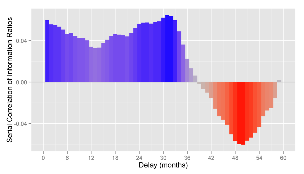
The chart below shows correlation between 12-month Information Ratios calculated with lags of one to sixty months (1-60 month delay):

Chart of the predictive power of information ratios as measured by their autocorrelation (the correlation between Information Ratios for one 12-month period and a different 12-month period separated by a given lag) for all U.S. equity 13F portfolios

13F Equity Portfolios: Serial correlation of Information Ratios

Delay (months) Serial Correlation
1 0.06
6 0.05
12 0.03
18 0.05
24 0.06
30 0.06
36 0.02
42 -0.02
48 -0.06
54 -0.04
60 0.02

Over the 3-year window, the serial correlation (autocorrelation) of Information Ratios is approximately half of the serial correlation of security selection returns provided in the following section. Unlike simple nominal returns and Sharpe ratios, information ratios do not suffer from short-term reversion.

Serial Correlation of Nominal Returns

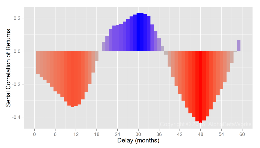
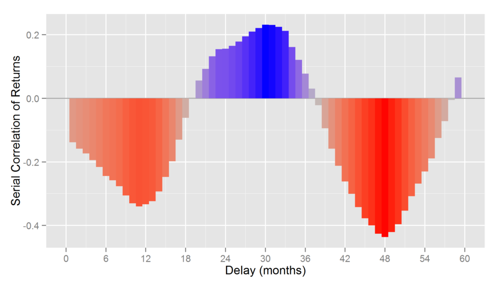
For comparison, the following chart shows serial correlation of 12-month cumulative nominal returns calculated with 1-60 month lags. As we discussed in prior articles, these revert with an approximately 18-month cycle – so strong past nominal returns are actually predictive of poor short-term future nominal returns:

Chart of the correlation between returns for one 12-month period and a different 12-month period separated by a given lag for all U.S. equity 13F portfolios

13F Equity Portfolios: Serial correlation of nominal returns

Delay (months) Serial Correlation
1 -0.14
6 -0.24
12 -0.33
18 -0.06
24 0.16
30 0.23
36 0.08
42 -0.26
48 -0.44
54 -0.23
60 0.13

Serial Correlation of Security Selection Returns

As we mentioned above, when a benchmark’s factor exposures match those of the portfolio, information ratio is equivalent to the standard score (z-score) of active returns estimated with a capable equity risk model. In practice, however, information ratio is typically calculated relative to a broad benchmark, such as the S&P 500 Index for equity portfolios. Consequently, one would expect the predictive power of information ratios to be lower than the predictive power of security selection returns, properly estimated. For comparison, we provide serial correlation of a security selection metric that uses an equity risk model to control for factor exposures.

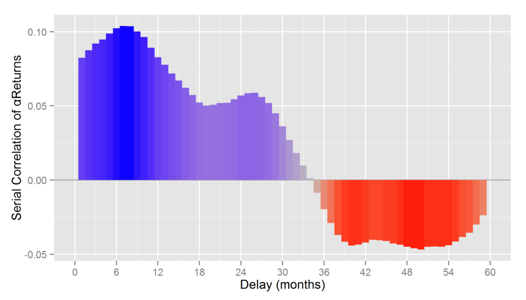
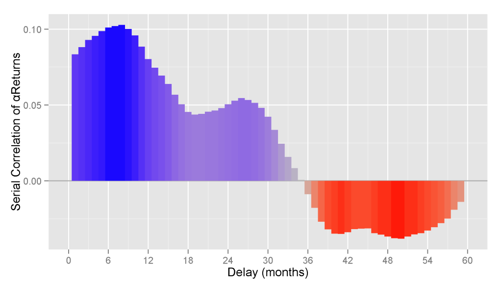
To eliminate the disruptive factor effects responsible for performance reversion, the AlphaBetaWorks Performance Analytics Platform calculates each portfolio’s return from security selection net of factor effects. αReturn is the return a portfolio would have generated if all factor returns had been zero. The following chart shows correlation between 12-month cumulative αReturns calculated with 1-60 month lags:

Chart of the correlation between αReturns (risk-adjusted returns from security selection) for one 12-month period and a different 12-month period separated by a given lag for all U.S. equity 13F portfolios

13F Equity Portfolios: Serial correlation of αReturns (risk-adjusted returns from security selection)

Delay (months) Serial Correlation
1 0.08
6 0.10
12 0.08
18 0.05
24 0.06
30 0.04
36 -0.02
42 -0.04
48 -0.05
54 -0.04
60 -0.02

The predictive power of αReturns, as measured by their serial correlation of 12-month performance metrics, is approximately twice that of information ratios over a 3-year window (12-month delay between 12-month performance metrics), but the two begin to converge after three years.

For all performance metrics, the above data is aggregate, spanning thousands of portfolios and return windows. Individual firms can overcome the averages; however, the exceptions require especially careful monitoring.

Summary

  • The predictive power of information ratios is significantly higher than that of nominal returns and Sharpe ratios.
  • As a benchmark converges to the factor exposures of a portfolio, information ratios converge to the standard score (z-score) of active returns estimated with a capable risk model.
  • Over a 3-year window, the predictive power of information ratios, as commonly calculated, is approximately half that of the security selection return calculated with a predictive equity risk model.
The information herein is not represented or warranted to be accurate, correct, complete or timely.
Past performance is no guarantee of future results.
Copyright © 2012-2016, AlphaBetaWorks, a division of Alpha Beta Analytics, LLC. All rights reserved.
Content may not be republished without express written consent.
U.S. Patents Pending

The Predictive Power of Sharpe Ratios

Our earlier work showed that performance metrics dominated by market noise, such as simple nominal returns, revert. Because of this reversion, above-average performers of the past tend to become below-average performers and vice versa. Since the reversion is primarily due to systematic (factor) noise, metrics that control for factor exposures reveal persistent stock picking skill. Prompted by readers’ questions, this series of articles will measure the predictive power of popular performance metrics. We first consider the predictive power of Sharpe Ratios. For the universe of all institutional U.S. long equity portfolios, the use of Sharpe Ratios for skill evaluation and manager selection is almost as damaging as the use of simple nominal returns.

Measuring the Predictive Power of Sharpe Ratios

We analyze portfolios of all institutions that have filed Forms 13F in the past 15 years. This survivorship-free portfolio dataset covers firms that have held as least $100 million in long U.S. assets. Approximately 5,000 portfolios had sufficiently long histories, low turnover, and broad holdings to be analyzable.

To measure the decay of performance metrics over time, we compare metrics measured in two 12-month periods separated by variable delay. One example of 24-month delay is metrics for 1/31/2010-1/31/2011 and 1/31/2013-1/31/2014. We use Spearman’s rank correlation coefficient to calculate statistically robust correlations.

Serial Correlation of Sharpe Ratios

Sharpe Ratio is perhaps the most common performance metric. Since it does not directly control for systematic (factor) portfolio exposures, one would expect this approach to suffer from similar reversion as nominal returns. Indeed, tests reveal that Sharpe Ratios fail to isolate security selection performance: Sharpe Ratios of portfolios revert when factor regimes change. Thus, former leaders tend to become laggards, and former laggards tend to become leaders.

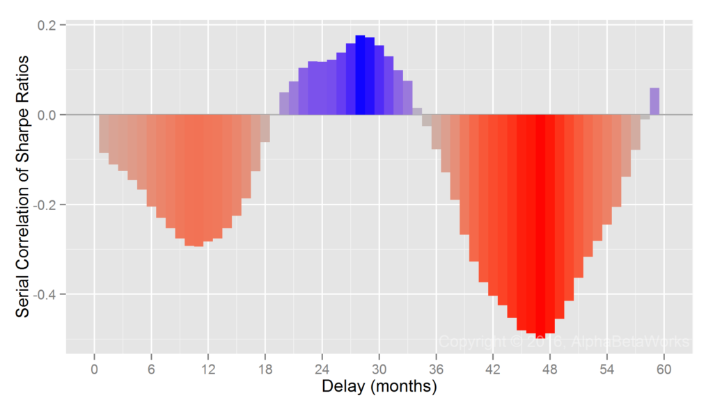
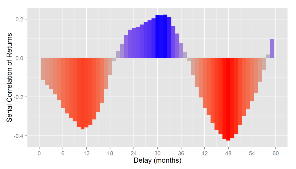
The serial correlation (autocorrelation) of Sharpe Ratios is similar to the serial correlation of nominal returns in the next section. The following chart shows correlation between 12-month Sharpe Ratios calculated with lags of one to sixty months (1-60 month lag):

The predictive power of Sharpe Ratios: Chart of the correlation between Sharpe Ratios for one 12-month period and a different 12-month period separated by a given lag for all U.S. equity 13F portfolios

13F Equity Portfolios: Serial correlation of Sharpe Ratios

Delay (months) Serial Correlation
1 -0.09
6 -0.20
12 -0.28
18 -0.06
24 0.12
30 0.15
36 -0.08
42 -0.40
48 -0.49
54 -0.24
60 0.12

Sharpe Ratios revert with an approximately 18-month cycle. Historical Sharpe Ratios thus have some predictive value, but a negative one. There is a narrow window at 2-3 year lag when past Sharpe Ratios are positively predictive of the future Sharpe Ratios. This is due to the approximately 18-month cycle of reversion.

Serial Correlation of Nominal Returns

For comparison, the following chart shows serial correlations between 12-month cumulative nominal returns calculated with 1-60 month lags. The relationship is similar to that of the Sharpe Ratios. Strong past (nominal) returns are predictive of poor short-term future returns:

Chart of the correlation between returns for one 12-month period and a different 12-month period separated by a given lag for all U.S. equity 13F portfolios

13F Equity Portfolios: Serial correlation of nominal returns

Delay (months) Serial Correlation
1 -0.14
6 -0.24
12 -0.33
18 -0.06
24 0.16
30 0.23
36 0.08
42 -0.26
48 -0.44
54 -0.23
60 0.13

Serial Correlation of Security Selection Returns

For additional comparison, we provide serial correlation of a security selection metric that adjusts for factor exposures. To eliminate the disruptive factor effects responsible for performance reversion, the AlphaBetaWorks Performance Analytics Platform calculates each portfolio’s return from security selection net of factor effects. αReturn is the return a portfolio would have generated if all factor returns had been flat. Firms with above-average αReturns in one period are likely to maintain them, though with a decay. The following chart shows correlation between 12-month cumulative αReturns calculated with 1-60 month lags:

Chart of the correlation between αReturns (risk-adjusted returns from security selection) for one 12-month period and a different 12-month period separated by a given lag for all U.S. equity 13F portfolios

13F Equity Portfolios: Serial correlation of αReturns (risk-adjusted returns from security selection)

Delay (months) Serial Correlation
1 0.08
6 0.10
12 0.08
18 0.05
24 0.06
30 0.04
36 -0.02
42 -0.04
48 -0.05
54 -0.04
60 -0.02

Though the above serial correlations of αReturn may appear low, they are amplified and compounded in practical portfolios of multiple funds. A hedged portfolio of the net consensus longs (relative overweights) of the top 5% long U.S. equity stock pickers delivered approximately 8% return independently of the market. The above data is aggregate. Specific outstanding disciplined firms can overcome performance reversion, but they are the exceptions that require careful monitoring.

Summary

  • Sharpe Ratios revert rapidly and are not significantly better predictors of future performance than nominal returns.
  • Once performance is controlled for systematic (factor) exposures, security selection returns persist for approximately 5 years.
  • Selection of superior future performers is possible, but it requires abandoning popular non-predictive metrics and spotting skill long before it is plainly visible and arbitraged away.
The information herein is not represented or warranted to be accurate, correct, complete or timely.
Past performance is no guarantee of future results.
Copyright © 2012-2016, AlphaBetaWorks, a division of Alpha Beta Analytics, LLC. All rights reserved.
Content may not be republished without express written consent.
U.S. Patents Pending

Tests of Equity Market Hedging: U.S. Mutual Funds

Equity market hedging techniques can be complex and their effectiveness hard to assess. In this piece we evaluate the effectiveness of several market hedging techniques by comparing them to the (idealized and unattainable) perfect market hedge. Specifically, we compare realized market correlations of hedged U.S. equity mutual fund portfolios to market correlations of random return series. Random return series are the ideal that would have been produced by perfect hedging of portfolios satisfying the random walk hypothesis. Whereas hedges that use a fixed 1 beta and hedges that use returns-based style analysis (RBSA) are flawed, a statistical equity risk model applied to portfolio holdings is close to the ideal.

Equity Market Hedging Techniques

We analyze approximately 3,000 non-index U.S. Equity Mutual Funds over 10 years. These provide a broad sample of the real-world long equity portfolios that investors may attempt to hedge. We evaluate the effectiveness of three techniques for calculating hedge ratios:

  • Assuming constant 100% market exposure (1 beta): Absent deeper statistical analysis, it is common to assume that all portfolios have the same market risk, equal to that of the broad benchmarks.
  • Using returns-based style analysis (RBSA): RBSA is a popular technique that attempts to estimate portfolio factor exposures by regressing portfolio returns against factor returns.
  • Applying a statistical equity risk model to portfolio holdings: This technique essentially performs RBSA on the individual portfolio holdings and aggregates the results.

For each fund and for each month of history we calculate market exposure at the end of the month and then use this estimated (ex-ante) exposure to hedge the fund during the following month. We then analyze realized (ex-post) 12-month hedged portfolio returns and calculate their correlations to the Market. The lower this correlation, the more effective a hedging technique is at eliminating systematic market exposure of a typical U.S. equity mutual fund portfolio.

Realized Market Correlations of Hedged U.S. Mutual Fund Portfolios

Realized Market Correlations of Random Return Series

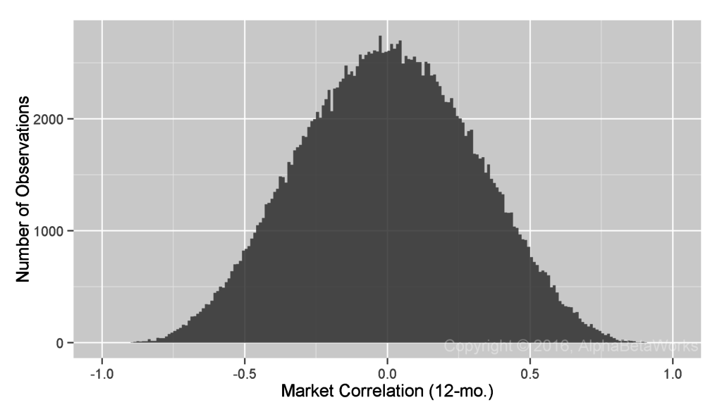
An effective hedging technique should produce zero mean and median market correlations of hedged portfolio returns. Yet, if sufficiently large, even a set of perfectly random 12-month return series will contain some with large market correlations. Since our study covers over 200,000 12-month samples (observations), some market correlations are close to 1 by mere chance. To account for this and to create a baseline for comparisons, we calculated market correlations for random return series with a Monte Carlo simulation. These results, attainable only with a perfect hedge, are the baseline against which we evaluate equity market hedging techniques:

Chart of the correlations between 12-month random return series and 12-month returns of U.S. Equity Market

Realized 12-month market correlations of random return series

    Min.    1st Qu.     Median       Mean    3rd Qu.       Max.
  -0.9243    -0.2162     0.0001    -0.0006     0.2146     0.9409

Realized Market Correlations of Portfolios Hedged using a 100% Market Short

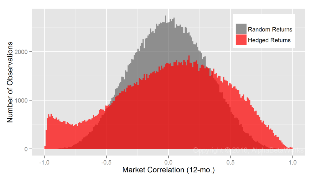
A naive assumption that market exposures of all portfolios are 100% (market betas of all portfolios are 1) is obviously wrong:

Chart of the correlations between realized 12-month returns of U.S. Equity Mutual Fund portfolios hedged using a 100% market short and 12-month returns of U.S. Equity Market

U.S. Equity Mutual Funds: Realized 12-month market correlations of portfolios hedged using a 100% market short

    Min.  1st Qu.   Median     Mean  3rd Qu.     Max. 
  -0.9956  -0.2927   0.0469   0.0148   0.3527   0.9958

This approach over-hedges some portfolios and under-hedges others. There is a group of low-exposure portfolios for which a fixed 100% market short is too large. These produce a fat tail of negative market correlations of nearly -1 for some hedged portfolios. There is also a group of portfolios for which a fixed 100% market hedge is too small.

Realized Market Correlations of Portfolios Hedged using Returns-Based Analysis

Returns-based style analysis with multiple factors suffers from known issues of overfitting and collinearity. Less well-known are the problems that arise from RBSA’s assumption that exposures are constant over the regression window. In practice, portfolio exposures vary over time and can change rapidly as positions change. RBSA will capture these changes months or even years later once they influence portfolio returns, if at all.

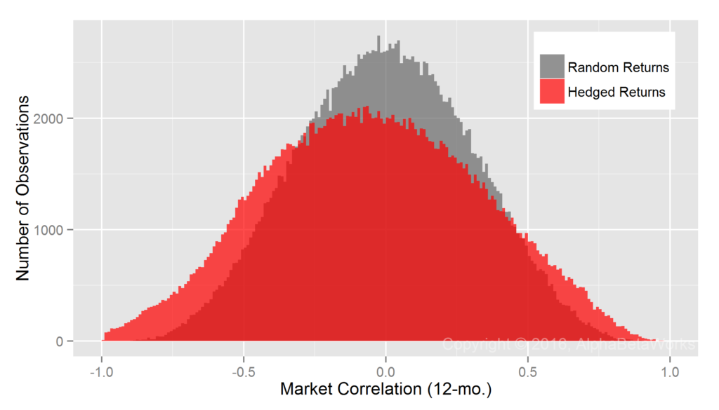
RBSA thus fails similarly to the fixed hedging above, if less dramatically: hedges are too large in some cases and too small in others. The exposure estimates are also apparently biased, since they produce hedges that are too large and market correlations that are negative, on average:

Chart of the correlations between realized 12-month returns of U.S. Equity Mutual Fund portfolios hedged using returns-based style analysis and 12-month returns of U.S. Equity Market

U.S. Equity Mutual Funds: Realized 12-month market correlations of portfolios hedged using returns-based style analysis

    Min.  1st Qu.   Median     Mean  3rd Qu.     Max. 
  -0.9946  -0.3229  -0.0518  -0.0459   0.2274   0.9762

Realized Market Correlations of Portfolios Hedged using a Statistical Equity Risk Model

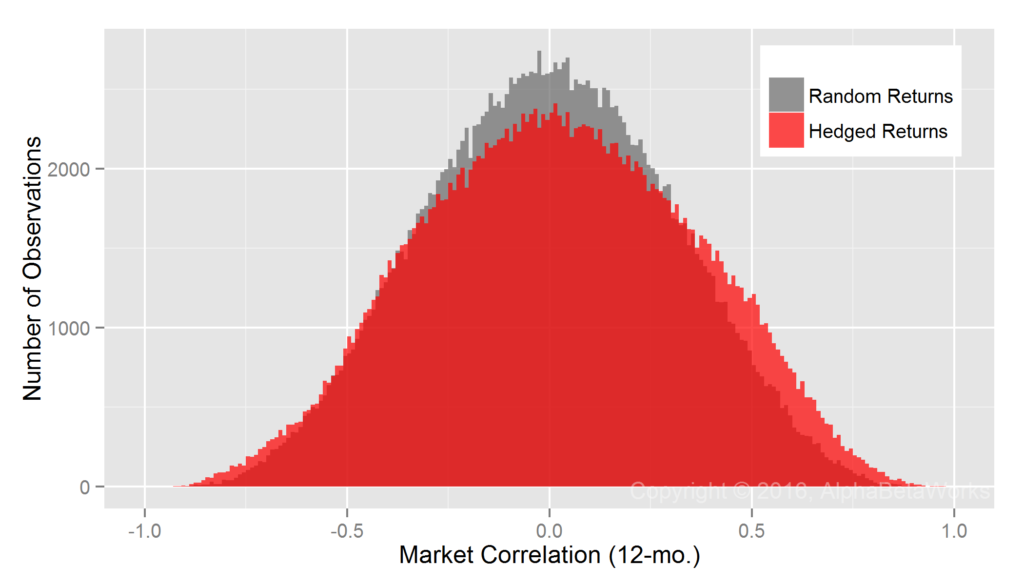
The AlphaBetaWorks Statistical Equity Risk Model produces hedges close to the ideal:

Chart of the correlations between realized 12-month returns of U.S. Equity Mutual Fund portfolios hedged using a statistical equity risk model applied to holdings and 12-month returns of U.S. Equity Market

U.S. Equity Mutual Funds: Realized 12-month market correlations of portfolios hedged using a statistical equity risk model applied to holdings

    Min.  1st Qu.   Median     Mean  3rd Qu.     Max. 
  -0.9565  -0.2230   0.0184   0.0214   0.2669   0.9755

The model estimates security market exposures using robust regression methods to control for outliers. Though robust techniques perform well for most portfolios, they appear to produce hedge ratios that are too low for some high-beta portfolios. This leads to small positive mean and median market correlations of hedged portfolio returns and to the higher probability of positive market correlations compared to random portfolios.

Aside from this under-hedging of a small fraction of portfolios, application of the AlphBetaWorks Statistical Equity risk model to fund holdings comes closest to perfect equity market hedging. Portfolio managers and investors who rely on robust risk models and hedging techniques can thus nearly perfectly hedge the market risk of a typical equity portfolio.

Summary

  • The effectiveness of equity market hedging techniques can be assessed by comparing hedged portfolio returns to random portfolio returns that would be produced by a perfect hedge.
  • Simplistic hedging that assumes 1 beta for all portfolios fails, most spectacularly for low-risk portfolios.
  • Returns-based style analysis (RBSA) both over-hedges and under-hedges, likely due to its failure to capture rapidly changing exposures.
  • Analysis of fund holdings using a Statistical Equity Risk Model comes closest to perfect equity market hedging.
The information herein is not represented or warranted to be accurate, correct, complete or timely.
Past performance is no guarantee of future results.
Copyright © 2012-2016, AlphaBetaWorks, a division of Alpha Beta Analytics, LLC. All rights reserved.
Content may not be republished without express written consent.

The Persistence of Negative Investment Performance

And why Poor Nominal Returns are a Reason to Hire Rather than Fire a Manager

Our earlier pieces discussed how nominal investment performance reverts. Since returns are dominated by systematic risk factors (primarily the Market), they are subject to reversal when investment regimes change. In the simplest terms, high risk funds do well in bull markets, and low risk funds do well in bear markets, irrespectively of stock picking skill. When the tide turns, so does the funds’ relative performance. The persistence of stock picking skill becomes evident once systematic effects are removed.

This piece focuses on the persistence of negative investment performance. Negative investment performance exacerbates the losses due to simplistic performance metrics and sharpens the edge of predictive skill analytics: Negative nominal returns revert more sharply than overall nominal returns; negative security selection returns persist longer.

Measuring Persistence of Investment Performance

As our prior performance persistence work, this study analyzes portfolios of all institutions that have filed Form 13F during the past 15 years. This survivorship-free portfolio database covers thousands of firms that have held at least $100 million in U.S. long assets during this period.

The relationship between performance metrics of a portfolio calculated at different points in time captures their persistence. To measure the persistence of nominal returns, we analyze nominal returns during two 12-month periods separated by variable delay. For example, analysis of 24-month delay includes periods 1/31/2010-1/31/2011 and 1/31/2013-1/31/2014. We use the Spearman’s rank correlation coefficient to calculate statistically robust correlations between metrics. Technically speaking, we are studying the metrics’ serial correlation or autocorrelation.

The Persistence of Investment Performance

The following charts of autocorrelation have been updated with data through 5/31/2016 and remain virtually unchanged from our earlier work on the decay of stock picking skill.

Serial Correlation of Nominal Returns

Portfolios with above-average nominal returns for prior 12 months tend to underperform for approximately the following two years; similarly, those with below average nominal returns tend to then outperform:

Chart of the persistence of stock picking performance as measured by the correlation between returns for one 12-month period and a different 12-month period separated by a given lag for all U.S. equity 13F portfolios

13F Equity Portfolios: Serial correlation of nominal returns

Delay (months) Serial Correlation
1 -0.11
6 -0.26
12 -0.36
18 -0.09
24 0.15
30 0.22
36 0.08
42 -0.26
48 -0.42
54 -0.22
60 0.17

Serial Correlation of Security Selection Returns

To eliminate the disruptive factor effects responsible for the above reversion, the AlphaBetaWorks Performance Analytics Platform calculates return from security selection after controlling for the factor exposures. The resulting metric, αReturn, is the return a portfolio would have generated if all factor returns had been flat. Above-average and below-average 12-month αReturns tend to persist for approximately four years:

Chart of the persistence of stock picking performance as measured by the correlation between <span style=

Delay (months) Serial Correlation
1 0.08
6 0.10
12 0.08
18 0.05
24 0.05
30 0.04
36 -0.01
42 -0.03
48 -0.04
54 -0.03
60 -0.01

The Persistence of Negative Investment Performance

The autocorrelation of overall nominal returns and αReturns captures the persistence of both negative and positive investment performance, but positive and negative metrics need not have similar persistence. In fact, the problems with nominal returns and simplistic performance metrics derived from them are accentuated when the nominal returns are negative.

Serial Correlation of Negative Nominal Returns

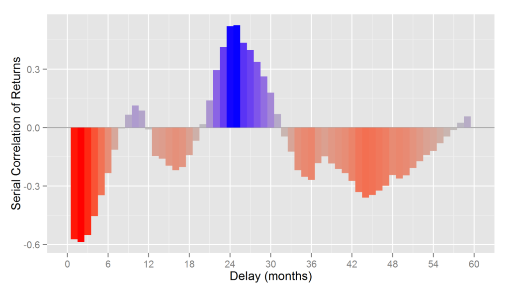
Negative 12-month nominal returns revert even more rapidly and more strongly than overall returns. Rank correlation coefficient for 12-month nominal returns separated by 6 months is approximately -0.5 for negative nominal returns and -0.2 for overall nominal returns. Poor recent nominal returns are a reason to hire rather than fire a manager, at least in the short term (the subsequent 12-18 months):

Chart of the persistence of negative investment performance as measured by the correlation between negative returns for one 12-month period and a different 12-month period separated by a given lag for all U.S. equity 13F portfolios

13F Equity Portfolios: Serial correlation of negative nominal returns

Delay (months) Serial Correlation
1 -0.57
6 -0.23
12 -0.01
18 -0.14
24 0.52
30 0.18
36 -0.27
42 -0.27
48 -0.24
54 -0.12
60 0.07

Serial Correlation of Negative Security Selection Returns

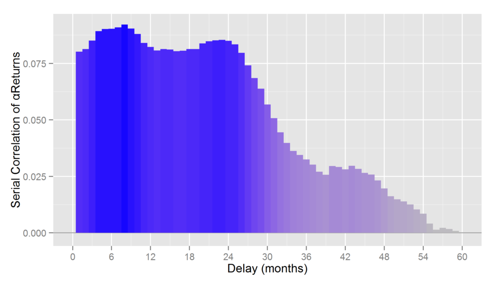
This reversion is not present for αReturns. Negative αReturns have similar autocorrelation for the first few years and decay more slowly than overall αReturns:

Chart of the persistence of negative investment performance as measured by the correlation between negative αReturns (risk-adjusted returns from security selection) for one 12-month period and a different 12-month period separated by a given lag for all U.S. equity 13F portfolios

13F Equity Portfolios: Serial correlation of αReturns (risk-adjusted returns from security selection)

Delay (months) Serial Correlation
1 0.08
6 0.09
12 0.08
18 0.08
24 0.08
30 0.06
36 0.03
42 0.03
48 0.02
54 0.01
60 0.00

The decay in security selection performance is typically due to such things as talent turnover, style drift, management distraction, and asset growth. Since these are more likely to affect the top-performing funds, negative αReturn remains predictive for longer. The above data is aggregate and specific firms can and do overcome the average fate. Though the above serial correlations may appear low, they are amplified and compounded in portfolios of multiple funds.

Cheerful consensus is usually a recipe for mediocrity, whether investing in a stock or in a fund. Fear and panic in the face of nominal underperformance are more dangerous still. Just as it pays to be a contrarian stock picker, it pays to be a contrarian fund investor or allocator.

Summary

  • Nominal returns and related simplistic metrics of investment skill revert rapidly.
  • Negative nominal returns revert more strongly than overall nominal returns.
  • Negative security selection performance persists longer than overall security selection performance.
  • When negative investment performance is merely nominal, it is a contrarian indicator.
  • When negative investment performance is due to poor security selection net of factor effects, it is a persistent and predictive indicator.
The information herein is not represented or warranted to be accurate, correct, complete or timely.
Past performance is no guarantee of future results.
Copyright © 2012-2016, AlphaBetaWorks, a division of Alpha Beta Analytics, LLC. All rights reserved.
Content may not be republished without express written consent.
U.S. Patents Pending

The Decay of Stock Picking Skill

Our earlier work showed that nominal returns and related simplistic performance metrics are dominated by market noise and hence revert. The reversion means that yesterday’s best-performing managers tend to be tomorrow’s worst. Yet, once distilled from systematic noise, stock picking skill is evident. This piece measures the decay of stock picking performance over time and identifies the historical window most predictive of future performance. We demonstrate that superior manager selection requires spotting skill well before the crowd arbitrages it away.

Measuring the Decay of Stock Picking Skill

This study analyzes portfolios of all institutions that have filed Form 13F. This is the broadest and most representative survivorship-free portfolio database covering thousands of firms that hold at least $100 million or more in U.S. long assets. Approximately 5,000 firms had sufficiently long histories, low turnover, and broad portfolios suitable for skill evaluation.

To measure the decay of stock picking performance over time, we compare metrics measured in two 12-month periods separated by variable delay. One example of 24-month delay is metrics for 1/31/2010-1/31/2011 and 1/31/2013-1/31/2014. We use Spearman’s rank correlation coefficient to calculate statistically robust correlations.

Serial Correlation of Nominal Returns

The following chart shows serial correlation (autocorrelation) between 12-month cumulative nominal returns calculated with lags of one to sixty months (1-60 month lag). The relationship is generally negative. This illustrates that strong past (nominal) returns are predictive of future returns, albeit poor in the short-term:

Chart of the decay of stock picking performance as measured by the correlation between returns for one 12-month period and a different 12-month period separated by a given lag for all U.S. equity 13F portfolios

13F Equity Portfolios: Serial correlation of nominal returns

Delay (months) Serial Correlation
1 -0.11
6 -0.26
12 -0.36
18 -0.09
24 0.15
30 0.22
36 0.08
42 -0.26
48 -0.42
54 -0.22
60 0.17

There is a narrow window at 2-3 year lag when past returns are predictive of the future results. This appears to be due to the approximately 18-month cycle of reversion in 12-month nominal performance.

Serial Correlation of Naive Alphas

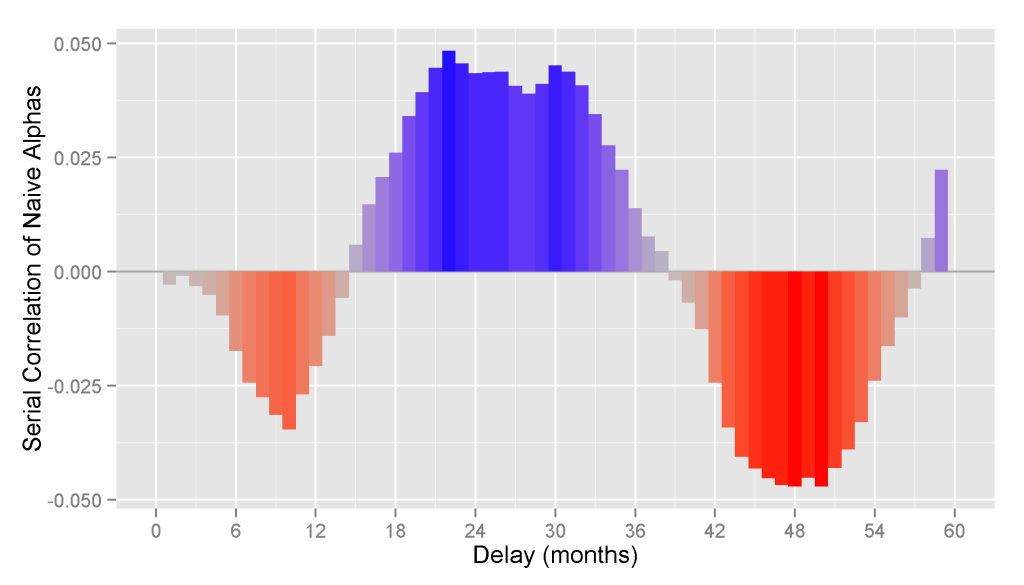
It is common to measure alpha simply as outperformance relative to a benchmark. We will call this approach “naive alpha.” Since it ignores portfolio risk, this approach does not eliminate systematic (factor) effects and fails to isolate security selection performance: The top nominal performers who took the most systematic risk in a bullish regime remain the top performers after a benchmark return is subtracted. When regimes change, these former leaders tend to become the laggards, and vice versa.

Indeed, the serial correlation of naive alphas is similar to the serial correlation of nominal returns. The following chart shows correlation between 12-month cumulative naive alphas calculated with 1-60 month lags:

Chart of the decay of stock picking performance as measured by the correlation between naïve alphas (returns over S&P 500) for one 12-month period and a different 12-month period separated by a given lag for all U.S. equity 13F portfolios

13F Equity Portfolios: Serial correlation of naive alphas (returns relative to the S&P 500 index)

Delay (months) Serial Correlation
1 0.00
6 -0.02
12 -0.02
18 0.03
24 0.04
30 0.05
36 0.01
42 -0.02
48 -0.05
54 -0.02
60 0.04

Serial Correlation of Security Selection Returns

To eliminate the disruptive factor effects responsible for performance reversion, the AlphaBetaWorks Performance Analytics Platform calculates each portfolio’s return from security selection net of factor effects. αReturn is the return a portfolio would have generated if all factor returns had been flat.

Firms with above-average αReturns in one period are likely to maintain them in the other, but with decay. The following chart shows correlation between 12-month cumulative αReturns calculated with 1-60 month lags:

Chart of the decay of stock picking performance as measured by the correlation between αReturns (risk-adjusted returns from security selection) for one 12-month period and a different 12-month period separated by a given lag for all U.S. equity 13F portfolios

13F Equity Portfolios: Serial correlation of αReturns (risk-adjusted returns from security selection)

Delay (months) Serial Correlation
1 0.08
6 0.10
12 0.08
18 0.05
24 0.05
30 0.04
36 -0.01
42 -0.03
48 -0.04
54 -0.03
60 -0.01

Though the above serial correlations of αReturn may appear low, they are amplified and compounded in practical portfolios of multiple funds. A hedged portfolio of the net consensus longs (relative overweights) of the top 5% long U.S. equity stock pickers delivered approximately 8% return independently of the market.

For approximately 3 years, strong security selection performance, as measured by the 12-month αReturn, is predictive of the future 12-month results. Returns due to security selection thus persist for approximately 5 years. This means that as little as 12 month of consistently positive αReturns are a positive indicator for the following four years. Skilled stock pickers can be spotted years before their skill is plainly visible and broadly exploited.

The decay in security selection performance is typically due to the following sources: talent turnover, style drift, management distraction, and asset growth. It is not a coincidence that the conventional requirement for large institutional allocation is 3-5 year track record.

The above data is aggregate. Specific outstanding disciplined firms can overcome this reversion, but they are the exceptions that require careful monitoring. Spotting skilled managers before their skill is visible to all is a sounder path to superior selection. In this respect, investing with managers is very similar to investing in stocks. Manager skill is arbitraged away – analytical advantage over the crowd is key. Cheerful consensus is usually a recipe for mediocrity whether investing in a stock or in a fund.

Summary

  • Nominal returns and related simplistic metrics of investment skill revert rapidly.
  • Security selection returns persist for approximately 5 years.
  • Selection of superior future performers is possible, but it requires spotting skill long before it is plainly visible and arbitraged away.
The information herein is not represented or warranted to be accurate, correct, complete or timely.
Past performance is no guarantee of future results.
Copyright © 2012-2016, AlphaBetaWorks, a division of Alpha Beta Analytics, LLC. All rights reserved.
Content may not be republished without express written consent.
U.S. Patents Pending.

Testing Global Equity Risk Models

Due to differences in financial reporting and transparency across international markets, fundamental company data is often unsuitable for building global risk models. Consequently, global equity risk models can be even more complex, brittle, and hard to interpret than their U.S. counterparts. Global statistical equity risk models are immune to these deficiencies in fundamental data and, when properly constructed to robustly capture the key risk factors, are highly predictive. An intuitive Global Statistical Equity Risk Model using Regional and Sector/Industry factors delivers over 0.96 correlation between predicted and reported portfolio returns for a median U.S. Equity Mutual Fund.

Predictive Power of Global Statistical Equity Risk Models

We analyze 10 years of historical positions and returns for over 3,000 non-index U.S. Equity Mutual Funds. The dataset spans domestic and international portfolios, extending our earlier test of U.S. equity risk models on domestic funds. We calculate factor exposures using estimated holdings at the end of each month and predict the next month’s performance using these ex-ante factor exposures and ex-post factor returns.

The correlation between an equity risk model’s predictions and subsequent performance illustrates the model’s power. High correlation indicates effectiveness at hedging, attributing returns to systematic sources, and evaluating manager skill. Global statistical equity risk models turn out to be even more effective than their U.S. counterparts.

Testing Predictions of Single-Factor Global Statistical Equity Risk Models

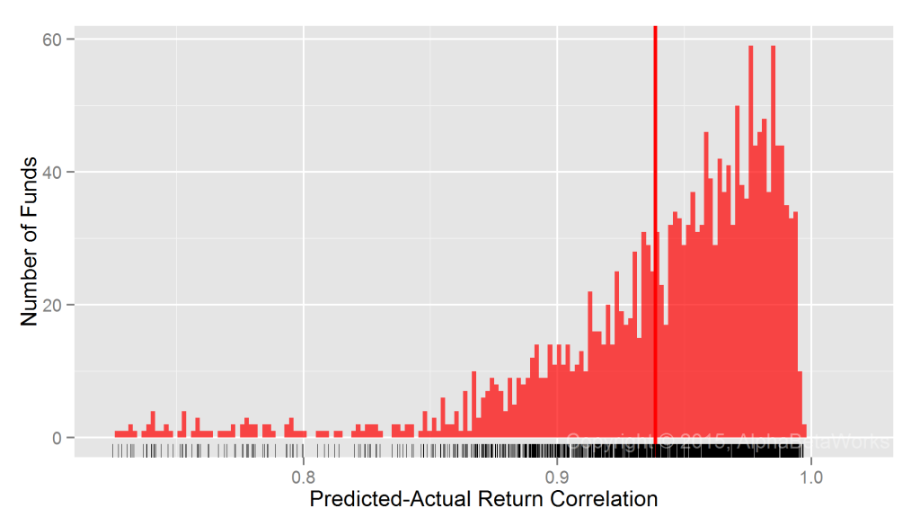
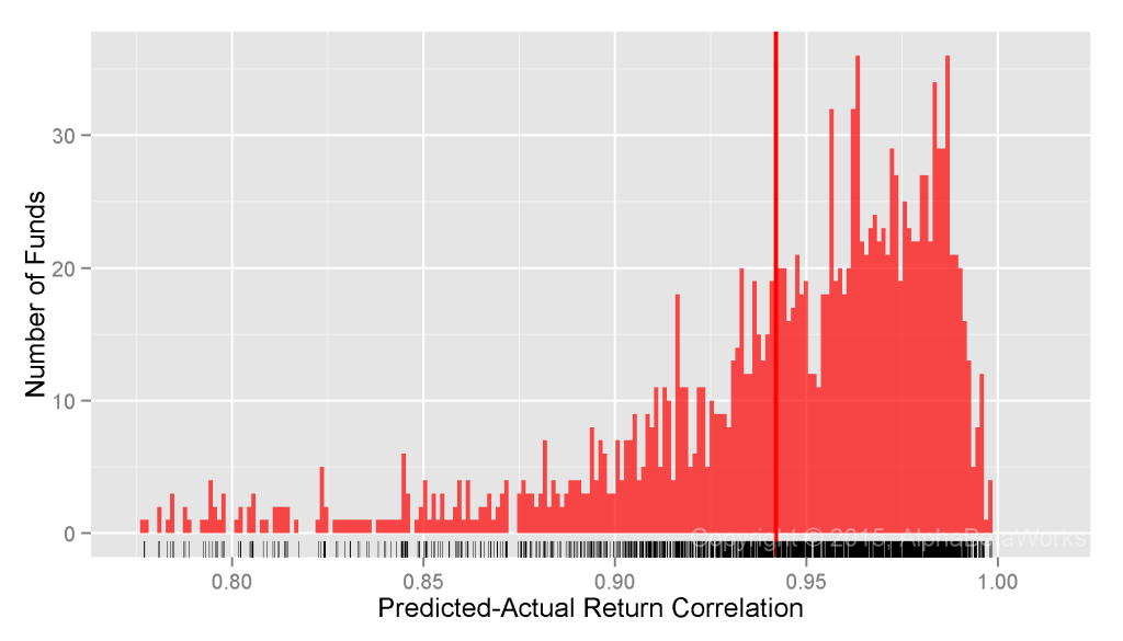
Our simplest global risk model uses a single systematic risk factor for each security – Region Beta. This factor is simply Market Beta for each of the 10 global regions such as North America, Developed Europe, and China. Since Market Beta is the dominant factor behind portfolio performance, even this simple model, when built with robust methods, delivers 0.94 mean and 0.95 median correlation between predicted and actual monthly returns:

Chart of the correlations between predicted returns constructed using a single-factor global statistical equity risk model and actual historical returns for U.S.-domiciled Global Equity Mutual Funds

Global U.S. Equity Mutual Funds: Correlation between a single-factor global statistical equity risk model’s predictions and actual monthly returns

   Min.    1st Qu. Median  Mean    3rd Qu. Max. 
   0.3881  0.9214  0.9540  0.9386  0.9758  0.9968

Testing Predictions of Two-Factor Global Statistical Equity Risk Models

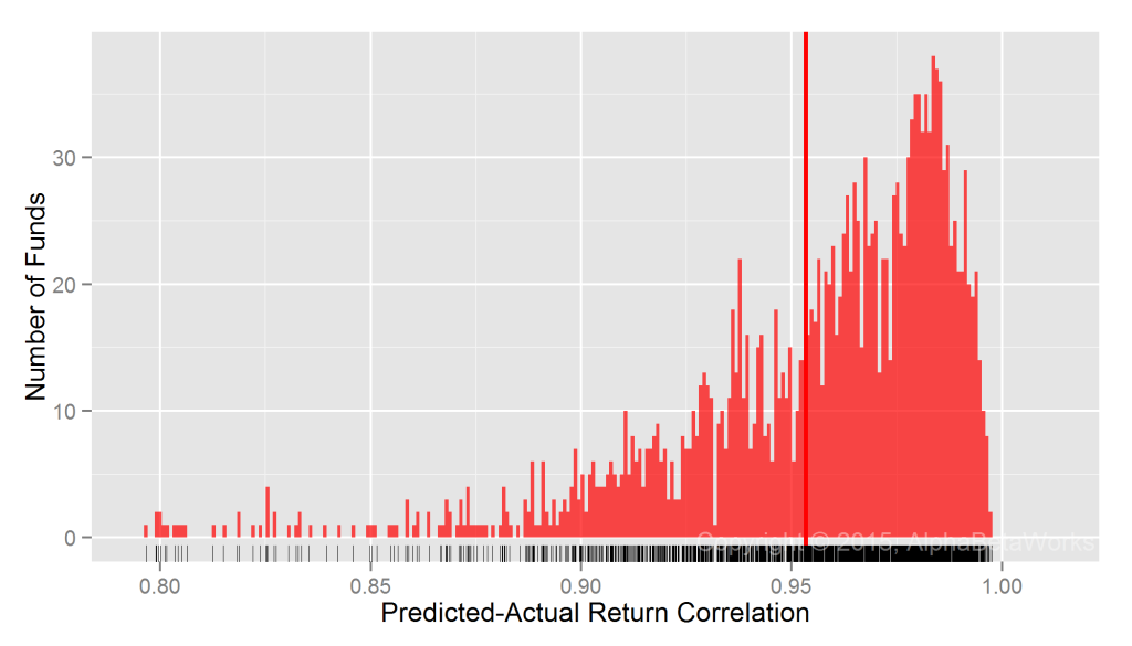
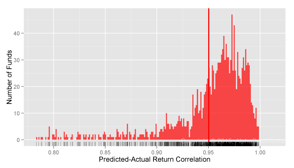
We now consider a two-factor model that adds a Sector Risk Factor. Each security belongs to one of 10 sectors such as Technology, Energy, or Utilities. Market and Sector Betas, estimated with robust methods, deliver 0.95 mean and over 0.96 median correlation between predicted and actual monthly returns:

Chart of the correlations between predicted returns constructed using a two-factor global statistical equity risk model and actual historical returns for U.S.-domiciled Global Equity Mutual Funds

Global U.S. Equity Mutual Funds: Correlation between a two-factor global statistical equity risk model’s predictions and actual monthly returns

  Min.    1st Qu. Median  Mean    3rd Qu. Max. 
  0.7030  0.9380  0.9647  0.9534  0.9809  0.9976

We picked sector as the second factor since research indicates that sector/industry performance captures more systematic portfolio risk than style factors do. Performance of common style factors can generally be explained by difference in sector composition of style portfolios. In contrast, performance of sectors cannot typically be attributed to differences in style of sector portfolios.

Even for the 25% funds the two-factor model handles the worst, the correlation between predicted and actual returns is 0.70-0.94. The lower accuracy of predictions is primarily caused by hybrid and fixed-income securities that are poorly described by an equity risk model.
Summary

  • Differences in financial reporting and transparency among countries make global equity risk model construction using fundamental data challenging and the resulting models fragile.
  • For a typical global U.S. mutual fund, even a minimalist statistical equity risk model with intuitive and investable factors delivers over 0.96 correlation between predicted and actual monthly returns.
  • An equity risk model with perfect prediction would, at most, improve correlation between predicted and actual returns by 0.035 and explain 6.9% more ex-post variance.
The information herein is not represented or warranted to be accurate, correct, complete or timely.
Past performance is no guarantee of future results.
Copyright © 2012-2015, AlphaBetaWorks, a division of Alpha Beta Analytics, LLC. All rights reserved.
Content may not be republished without express written consent.

Testing Predictions of Equity Risk Models

Equity risk models can be complex and hard to interpret. Yet, when properly constructed, robust statistical equity risk models capturing just the most salient factors are highly predictive. For instance, Market and Sector/Industry factors alone deliver 0.96 median correlation between predictions of equity risk models and reported portfolio returns for U.S. Equity Mutual Funds.

Predictive Power of Statistical Equity Risk Models

We analyze historical positions and returns of approximately 3,000 non-index U.S. Equity Mutual Funds over 10 years. We calculate factor exposures using estimated holdings at the end of each month and predict next month’s performance using these ex-ante factor exposures and ex-post factor returns.

The correlation between an equity risk model’s predictions and subsequently reported fund returns illustrates the model’s power. The higher the correlation, the more effective a model is at hedging, attributing returns to systematic sources, and evaluating manager skill.

Testing Predictions of Single-Factor Statistical Equity Risk Models

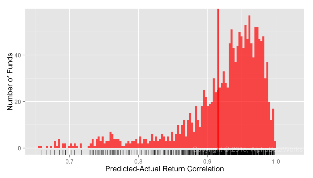
The simplest statistical equity risk model uses a single systematic risk factor – Market Beta. Since Market Beta is the dominant factor behind portfolio performance, even a very simple model built with robust methods delivers 0.92 mean and 0.94 median correlation between predicted and actual monthly returns:

Chart of the correlations between predicted returns constructed using a single-factor statistical equity risk model and actual historical returns for U.S. Equity Mutual Funds

U.S. Equity Mutual Funds: Correlation between a single-factor statistical equity risk model’s predictions and actual monthly returns

  Min.    1st Qu. Median  Mean    3rd Qu. Max. 
  0.1360  0.9010  0.9401  0.9157  0.9650  0.9981

Testing Predictions of Two-Factor Statistical Equity Risk Models

Research indicates that sector/industry risk factors capture more systematic portfolio risk than style factors do. For instance, in periods such as 1999-2001 the performance of common style factors is due to difference in sector composition of style portfolios.

Thus, we consider a two-factor model that adds a Sector Risk Factor. Each security belongs to one of 10 sectors. Market and Sector Betas, estimated with robust methods delivers 0.94 mean and 0.96 median correlation between predicted and actual monthly returns:

Chart of the correlations between predicted returns constructed using a two-factor statistical equity risk model and actual historical returns for U.S. Equity Mutual Funds

U.S. Equity Mutual Funds: Correlation between a two-factor statistical equity risk model’s predictions and actual monthly returns

  Min.    1st Qu. Median  Mean    3rd Qu. Max. 
  0.6639  0.9254  0.9562  0.9420  0.9753  0.9984

Testing Predictions of Multi-Factor Statistical Equity Risk Models

With correlation between predicted and actual returns very close to 1, the benefit of increased model complexity is rapidly diminishing. Even a perfect model would, at most, provide 0.0438 higher correlation, or explain 0.0857 higher fraction of ex-post variance for most funds than the above two-factor model.

Extending the two-factor model with Style Factors (Value/Growth and Size) as well as Macroeconomic Factors (Bonds, Oil, Currency, etc.), we arrive at the AlphaBetaWorks’ U.S. Equity Statistical Risk Model. It delivers 0.95 mean and 0.96 median correlation between predicted and actual monthly returns for U.S. Equity Mutual Funds:

Chart of the correlations between predicted returns constructed using a multi-factor statistical equity risk model and actual historical returns for U.S. Equity Mutual Funds

U.S. Equity Mutual Funds: Correlation between a multi-factor statistical equity risk model’s predictions and actual monthly returns

  Min.    1st Qu. Median  Mean    3rd Qu. Max. 
  0.6661  0.9420  0.9629  0.9503  0.9766  0.9987

Even for the 25% funds it handles the worst, the model delivers 0.67-0.94 correlation between predicted and actual returns.

Summary

  • Complex equity risk models with non-intuitive factors may offer no better predictions than robust models with a few intuitive factors.
  • Even a perfect equity risk model would, at most, explain 8.6% more ex-post variance than a simple two-factor model.
  • For a typical U.S. mutual fund, a statistical equity risk model with intuitive and investable factors delivers over 0.96 correlation between predicted and actual monthly returns.
The information herein is not represented or warranted to be accurate, correct, complete or timely.
Past performance is no guarantee of future results.
Copyright © 2012-2015, AlphaBetaWorks, a division of Alpha Beta Analytics, LLC. All rights reserved.
Content may not be republished without express written consent.