Our earlier work showed that simple performance metrics, such as nominal returns and Sharpe Ratios, revert. Because of this reversion, above-average past performers tend to become below-average and vice versa. This reversion is primarily due to systematic (factor) noise. Consequently, metrics that remove factor effects from performance reveal persistent stock picking skill. Prompted by readers’ questions, we have investigated the predictive power of popular performance metrics. This article reviews the predictive power of information ratios. They offer a large improvement over simple nominal returns, naive alphas, and Sharpe ratios, but still fall short of the most predictive metrics. Over a 3-year window, the predictive power of information ratios for skill evaluation and manager selection is approximately half that of security selection distilled with a statistical equity risk model.
Measuring the Predictive Power of Information Ratios
We analyze portfolios of all institutions that have filed Forms 13F in the past 15 years. This survivorship-free portfolio dataset covers firms that have held as least $100 million in long U.S. assets. Approximately 5,000 portfolios had sufficiently long histories and low turnover to be analyzable.
To measure the persistence of performance metrics over time, we compare metrics measured in two 12-month periods separated by variable delay. One example is the 24-month delay that separates metrics for 1/31/2010-1/31/2011 and 1/31/2013-1/31/2014. A 24-month delay of 12-month metrics thus covers a 48-month time window. We use Spearman’s rank correlation coefficient to calculate statistically robust correlations.
Serial Correlation of Information Ratios
The information ratio is similar to the Sharpe ratio, but with a key upgrade: Sharpe ratio evaluates returns relative to the risk-free rate. Information ratio evaluates returns relative to a (presumably appropriate) benchmark. We use the S&P 500 Index as the benchmark, following a common practice. As a benchmark increasingly matches the factor exposures of a portfolio, information ratios converge to the standard score (z-score) of active returns estimated with a capable equity risk model. Due to the more effective handling of systematic risk, the predictive power of information ratios receives a boost.
The chart below shows correlation between 12-month Information Ratios calculated with lags of one to sixty months (1-60 month delay):

13F Equity Portfolios: Serial correlation of Information Ratios
| Delay (months) | Serial Correlation |
| 1 | 0.06 |
| 6 | 0.05 |
| 12 | 0.03 |
| 18 | 0.05 |
| 24 | 0.06 |
| 30 | 0.06 |
| 36 | 0.02 |
| 42 | -0.02 |
| 48 | -0.06 |
| 54 | -0.04 |
| 60 | 0.02 |
Over the 3-year window, the serial correlation (autocorrelation) of Information Ratios is approximately half of the serial correlation of security selection returns provided in the following section. Unlike simple nominal returns and Sharpe ratios, information ratios do not suffer from short-term reversion.
Serial Correlation of Nominal Returns
For comparison, the following chart shows serial correlation of 12-month cumulative nominal returns calculated with 1-60 month lags. As we discussed in prior articles, these revert with an approximately 18-month cycle – so strong past nominal returns are actually predictive of poor short-term future nominal returns:

13F Equity Portfolios: Serial correlation of nominal returns
| Delay (months) | Serial Correlation |
| 1 | -0.14 |
| 6 | -0.24 |
| 12 | -0.33 |
| 18 | -0.06 |
| 24 | 0.16 |
| 30 | 0.23 |
| 36 | 0.08 |
| 42 | -0.26 |
| 48 | -0.44 |
| 54 | -0.23 |
| 60 | 0.13 |
Serial Correlation of Security Selection Returns
As we mentioned above, when a benchmark’s factor exposures match those of the portfolio, information ratio is equivalent to the standard score (z-score) of active returns estimated with a capable equity risk model. In practice, however, information ratio is typically calculated relative to a broad benchmark, such as the S&P 500 Index for equity portfolios. Consequently, one would expect the predictive power of information ratios to be lower than the predictive power of security selection returns, properly estimated. For comparison, we provide serial correlation of a security selection metric that uses an equity risk model to control for factor exposures.
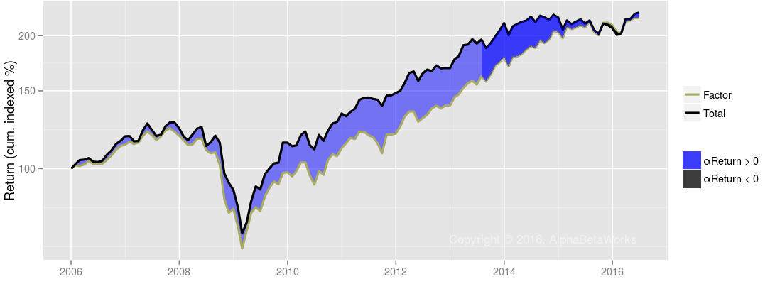
To eliminate the disruptive factor effects responsible for performance reversion, the AlphaBetaWorks Performance Analytics Platform calculates each portfolio’s return from security selection net of factor effects. αReturn is the return a portfolio would have generated if all factor returns had been zero. The following chart shows correlation between 12-month cumulative αReturns calculated with 1-60 month lags:

13F Equity Portfolios: Serial correlation of αReturns (risk-adjusted returns from security selection)
| Delay (months) | Serial Correlation |
| 1 | 0.08 |
| 6 | 0.10 |
| 12 | 0.08 |
| 18 | 0.05 |
| 24 | 0.06 |
| 30 | 0.04 |
| 36 | -0.02 |
| 42 | -0.04 |
| 48 | -0.05 |
| 54 | -0.04 |
| 60 | -0.02 |
The predictive power of αReturns, as measured by their serial correlation of 12-month performance metrics, is approximately twice that of information ratios over a 3-year window (12-month delay between 12-month performance metrics), but the two begin to converge after three years.
For all performance metrics, the above data is aggregate, spanning thousands of portfolios and return windows. Individual firms can overcome the averages; however, the exceptions require especially careful monitoring.
Summary
- The predictive power of information ratios is significantly higher than that of nominal returns and Sharpe ratios.
- As a benchmark converges to the factor exposures of a portfolio, information ratios converge to the standard score (z-score) of active returns estimated with a capable risk model.
- Over a 3-year window, the predictive power of information ratios, as commonly calculated, is approximately half that of the security selection return calculated with a predictive equity risk model.